Thực hành huấn luyện Audio Classification model

Đây là bài thứ 4 trong chuỗi 5 bài về Audio Deep Learning. Trong bài này, chúng ta sẽ code thực hành huấn luyện một mô hình phân loại Audio. Chúng ta sẽ đi tuần tự từng bước, từ việc chuẩn bị dữ liệu, xây dựng kiến trúc model, huấn luyện và đánh giá model. Cuối cùng là sử dụng model đã huấn luyện để dự đoán. Một số hướng mở rộng để nâng cao độ chính xác của model cũng sẽ được đưa ra bàn thảo.
1. Luồng hoạt động của bài toán Audio Classification
Tương tự như bài toán Image Classification hay Text Classification, bài toán Audio Classification thông thường sẽ bao gồm các bước xử lý chính như sau:
- Dữ liệu Audio được chuyển sang dạng Spectrogram (hoặc Mel Spectrogram, hoặc MFCC).
- Spectrogram Image được đưa qua mạng CNN để tạo ra Feature Maps.
- Sử dụng Feature Maps làm đầu vào cho bộ phân lớp (FC, SVM, …) để cho ra kết qủa dự đoán.

2. Chuẩn bị dữ liệu
2.1 Download dữ liệu
Chúng ta sẽ sử dụng bộ dữ liệu Urban Sound 8K trong bài này. Nó bao gồm 10 classes là các loại âm thanh khác nhau như tiếng chó sủa, tiếng còi báo động, tiếng mát khoan, …
Sau khi tải về, chúng ta thấy bộ dữ liệu này gồm 2 phần:
- Các Audio files trong 10 sub-folders có tên từ fold1 đến fold10. Trong mỗi sub-folders đó đều chứa các Audio files. Ví dụ: fold1/103074-7-1-0.wav. Độ dài của mỗi file Audio khoảng 4s.
- File UrbanSound8K.csv chứa thông tin về mỗi Audio files trong bộ dữ liệu: Tên file, nhãn, … Nhãn của mỗi file Audio được quy định là theo ID từ 0 đến 9.
2.2 Tiền xử lý dữ liệu
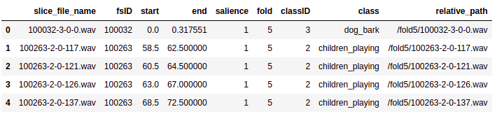
Mọi thông tin về dataset đều nằm trong file UrbanSound8K.csv (metadata file), vì vậy, trước tiên chúng ta đọc nó lên dể xem nó chứa những thông tin gì:
# ----------------------------
# Prepare training data from Metadata file
# ----------------------------
import pandas as pd
from pathlib import Path

data_path = '/home/sunt/Downloads/UrbanSound8k'

# Read metadata file
metadata_file = download_path + '/UrbanSound8K.csv'
df = pd.read_csv(metadata_file)
df.head()

# Construct file path by concatenating fold and file name
df['relative_path'] = '/fold' + df['fold'].astype(str) + '/' + df['slice_file_name'].astype(str)

# Take relevant columns
# df = df[['relative_path', 'classID']]
df.head()
Tiếp theo, chúng ta sẽ thực hiện một số bước tiền xử lý (pre-processing) dữ liệu để sẵn sàng đưa vào model huấn luyện. Quá trình Pre-processing sẽ đuợc thực hiện một cách tự động, cùng lúc với việc đọc các files Audio (thực hiện lúc runtime). Nói một cách dễ hiểu là đọc files Audio đến đâu, thực hiện Pre-processing và đưa vào model huấn luyện đến đó chứ không phải đọc xong toàn bộ files Audio rồi mới thực hiện các bước kia. Cách làm này cũng tương tự như cách chúng ta thường làm với dữ liệu Image, bởi vì cả 2 loại dữ liệu này thường tương đối lớn, nếu đọc hết một lần thì sẽ rất tốn bộ nhớ. Tất nhiên, vì model yêu cầu nhận vào dữ liệu theo từng Batch nên chúng ta cũng sẽ đọc và tiền xử lý dữ liệu theo từng Batch. Như vậy thì trong bộ nhớ lúc nào cũng chỉ có tối đa một Batch dữ liệu, tránh được việc tràn bộ nhớ. Giá trị của Batch, gọi là Batch_size có thể lớn hoặc nhỏ tùy theo kích thước bộ nhớ máy tính xử lý của bạn.

Ở bài này, mình sẽ sử dụng Pytorch và thư việ torchaudio để thực hiện. Code cho từng bước lần lượt như sau:
- Đọc Audio files
import math, random
import torch
import torchaudio
from torchaudio import transforms
from IPython.display import Audio

class AudioUtil():
   # ----------------------------
   # Load an audio file. Return the signal as a tensor and the sample rate
   # ----------------------------
   @staticmethod
   def open(audio_file):
      sig, sr = torchaudio.load(audio_file)
      return (sig, sr)
- Convert to two channels
Một vài files Audio có thể ở dạng một kênh (mono), trong khi đó một số khác ở dạng hai kênh (stereo). Bởi vì model chỉ chấp nhận dữ liệu có cùng kích thước nên chúng ta sẽ chuyển đổi tất cả sang dạng stereo:
# ----------------------------
# Convert the given audio to the desired number of channels
# ----------------------------
@staticmethod
def rechannel(aud, new_channel):
   sig, sr = aud

   if (sig.shape[0] == new_channel):
      # Nothing to do
      return aud

   if (new_channel == 1):
      # Convert from stereo to mono by selecting only the first channel
      resig = sig[:1, :]
   else:
      # Convert from mono to stereo by duplicating the first channel
      resig = torch.cat([sig, sig])

   return ((resig, sr))
- Standardize sampling rate
Tương tự bước thứ 2, các files Audio có thể có Sample Rate khác nhau (48000Hz, 44100Hz, …). Chúng ta phải đưa tất cả về cùng 1 giá trị của Sample Rate:
# ----------------------------
# Since Resample applies to a single channel, we resample one channel at a time
# ----------------------------
@staticmethod
def resample(aud, newsr):
   sig, sr = aud

   if (sr == newsr):
      # Nothing to do
      return aud

   num_channels = sig.shape[0]
   # Resample first channel
   resig = torchaudio.transforms.Resample(sr, newsr)(sig[:1,:])
   if (num_channels > 1):
      # Resample the second channel and merge both channels
      retwo = torchaudio.transforms.Resample(sr, newsr)(sig[1:,:])
      resig = torch.cat([resig, retwo])

   return ((resig, newsr))
- Resize to the same length
Tiếp tục, chúng ta sẽ thay đổi chiều dài của tất cả các files Audio về chung một giá trị max_length. File có chiều dài nhỏ hơn max_length sẽ được kéo dài bằng cách thêm vào khoảng im lặng - slience. File có chiều dài lớn hơn max_length sẽ được cắt bớt đi.
# ----------------------------
# Pad (or truncate) the signal to a fixed length 'max_ms' in milliseconds
# ----------------------------
@staticmethod
def pad_trunc(aud, max_ms):
   sig, sr = aud
   num_rows, sig_len = sig.shape
   max_len = sr//1000 * max_ms

   if (sig_len > max_len):
      # Truncate the signal to the given length
      sig = sig[:,:max_len]

   elif (sig_len < max_len):
      # Length of padding to add at the beginning and end of the signal
      pad_begin_len = random.randint(0, max_len - sig_len)
      pad_end_len = max_len - sig_len - pad_begin_len

      # Pad with 0s
      pad_begin = torch.zeros((num_rows, pad_begin_len))
      pad_end = torch.zeros((num_rows, pad_end_len))

      sig = torch.cat((pad_begin, sig, pad_end), 1)

   return (sig, sr)
- Data Augmentation: Time Shift
Đến đây, chúng ta đã coi như thực hiện Pre-processing xong dữ liệu thô của Audio. Chúng ta có thể áp dụng kỹ thuật Augmentation ở tại bước này, cụ thể là Time-Shift.
# ----------------------------
# Shifts the signal to the left or right by some percent. Values at the end
# are 'wrapped around' to the start of the transformed signal.
# ----------------------------
@staticmethod
def time_shift(aud, shift_limit):
   sig,sr = aud
   _, sig_len = sig.shape
   shift_amt = int(random.random() * shift_limit * sig_len)
   return (sig.roll(shift_amt), sr)
Ngoài Time-Shift, vẫn còn một số kỹ thuật Augmentation khác có thể áp dụng ở đây. Bạn có thể xem lại ở bài số 3 tại đây.
- Convert to Mel Spectrogram
Dữ liệu Audio thô sau đó sẽ được chuyển sang dạng Mel Spectrogram. Bạn có thể xem lại lý thuyết về Mel Spectrogram và lý do cần chuyển sang Mel Spectrogram ở bài số 2 tại đây
# ----------------------------
# Generate a Spectrogram
# ----------------------------
@staticmethod
def spectro_gram(aud, n_mels=64, n_fft=1024, hop_len=None):
   sig,sr = aud
   top_db = 80

   # spec has shape [channel, n_mels, time], where channel is mono, stereo etc
   spec = transforms.MelSpectrogram(sr, n_fft=n_fft, hop_length=hop_len, n_mels=n_mels)(sig)

   # Convert to decibels
   spec = transforms.AmplitudeToDB(top_db=top_db)(spec)
   return (spec)
- Data Augmentation: Time and Frequency Masking
Tiếp tục áp dụng thêm một số kỹ thuật Augmentation nữa đối với Mel Spectrogram. Lần này là SpecAugment với 2 phương pháp Time and Frequency Masking.
# ----------------------------
# Augment the Spectrogram by masking out some sections of it in both the frequency
# dimension (ie. horizontal bars) and the time dimension (vertical bars) to prevent
# overfitting and to help the model generalise better. The masked sections are
# replaced with the mean value.
# ----------------------------
@staticmethod
def spectro_augment(spec, max_mask_pct=0.1, n_freq_masks=1, n_time_masks=1):
   _, n_mels, n_steps = spec.shape
   mask_value = spec.mean()
   aug_spec = spec

   freq_mask_param = max_mask_pct * n_mels
   for _ in range(n_freq_masks):
      aug_spec = transforms.FrequencyMasking(freq_mask_param)(aug_spec, mask_value)

   time_mask_param = max_mask_pct * n_steps
   for _ in range(n_time_masks):
      aug_spec = transforms.TimeMasking(time_mask_param)(aug_spec, mask_value)

   return aug_spec
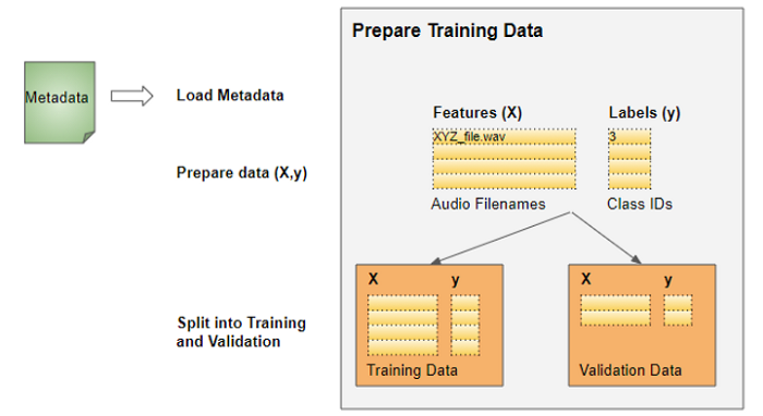
3. Định nghĩa Data Set và Data Loader
Để đưa dữ liệu vào cho model để huẩn luyện, trong Pytorch, chúng ta cần 2 Objects:
- Dataset object: Sử dụng tất cả các hàm Pre-processing đã định nghĩa ở trên.
from torch.utils.data import DataLoader, Dataset, random_split
import torchaudio

# ----------------------------
# Sound Dataset
# ----------------------------
class SoundDS(Dataset):
   def __init__(self, df, data_path):
      self.df = df
      self.data_path = str(data_path)
      self.duration = 4000
      self.sr = 44100
      self.channel = 2
      self.shift_pct = 0.4

   # ----------------------------
   # Number of items in dataset
   # ----------------------------
   def __len__(self):
      return len(self.df)

   # ----------------------------
   # Get i'th item in dataset
   # ----------------------------
   def __getitem__(self, idx):
      # Absolute file path of the audio file - concatenate the audio directory with
      # the relative path
      audio_file = self.data_path + self.df.loc[idx, 'relative_path']
      # Get the Class ID
      class_id = self.df.loc[idx, 'classID']

      aud = AudioUtil.open(audio_file)
      # Some sounds have a higher sample rate, or fewer channels compared to the
      # majority. So make all sounds have the same number of channels and same
      # sample rate. Unless the sample rate is the same, the pad_trunc will still
      # result in arrays of different lengths, even though the sound duration is
      # the same.
      reaud = AudioUtil.resample(aud, self.sr)
      rechan = AudioUtil.rechannel(reaud, self.channel)

      dur_aud = AudioUtil.pad_trunc(rechan, self.duration)
      shift_aud = AudioUtil.time_shift(dur_aud, self.shift_pct)
      sgram = AudioUtil.spectro_gram(shift_aud, n_mels=64, n_fft=1024, hop_len=None)
      aug_sgram = AudioUtil.spectro_augment(sgram, max_mask_pct=0.1, n_freq_masks=2, n_time_masks=2)

      return aug_sgram, class_id
- DataLoader object: Sử dụng Dataset object để lấy ra từng dữ liệu, gom thành từng Batch trước khi đưa cho model học.
Toàn bộ dữ liệu sẽ được chia thành 2 phần train/validation theo tỷ lệ 80/20, sau đó được sử dụng để tạo ra các DataLoader.
from torch.utils.data import random_split

myds = SoundDS(df, data_path)

# Random split of 80:20 between training and validation
num_items = len(myds)
num_train = round(num_items * 0.8)
num_val = num_items - num_train
train_ds, val_ds = random_split(myds, [num_train, num_val])

# Create training and validation data loaders
train_dl = torch.utils.data.DataLoader(train_ds, batch_size=16, shuffle=True)
val_dl = torch.utils.data.DataLoader(val_ds, batch_size=16, shuffle=False)
Mỗi Batch sẽ bao gồm 2 Tensors, một là Mel Spectrogram và một là nhãn tương ứng. Các Batch được lấy ngẫu nhiên từ tập train thông qua các Epoch. Kích thước của Batch sẽ là: (batch_size, num_chanels, Mel freq_bands, time_steps).

Nếu chúng ta thử Visualize một Data Sample trong một Batch lên sẽ được như sau:
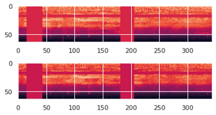
Ta có thể thấy các đường sọc ngang, dọc. Đó là kết quả của việc áp dụng các kỹ thuật SpecAugment.
Dữ liệu bây giờ đã sẵn sàng để đưa cho model học tập.
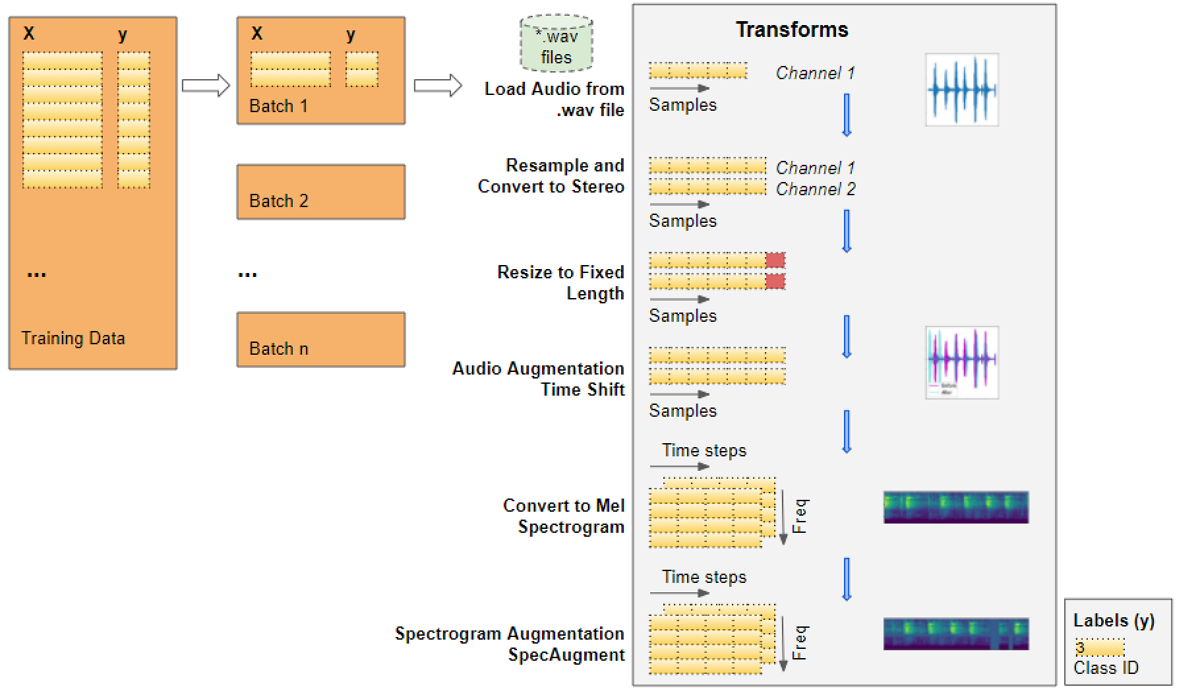
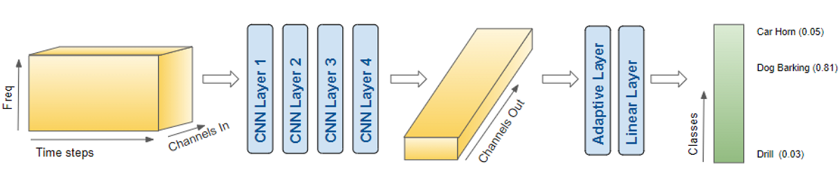
Toàn bộ quá trình Pre-precessing thông qua Dataset và DataLoader được thể hiện như trong hình dưới đây:
4. Tạo model
Bởi vì dữ liệu huấn luyện là Mel Spectrogram có dạng Image nên chúng ta sẽ xây dựng model bằng cách kết hợp một vài lớp CNN để trích xuất đặc trưng của ảnh và một vài lớp FC làm nhiệm vụ phân loại.
import torch.nn.functional as F
from torch.nn import init

# ----------------------------
# Audio Classification Model
# ----------------------------
class AudioClassifier (nn.Module):
    # ----------------------------
    # Build the model architecture
    # ----------------------------
    def __init__(self):
        super().__init__()
        conv_layers = []

        # First Convolution Block with Relu and Batch Norm. Use Kaiming Initialization
        self.conv1 = nn.Conv2d(2, 8, kernel_size=(5, 5), stride=(2, 2), padding=(2, 2))
        self.relu1 = nn.ReLU()
        self.bn1 = nn.BatchNorm2d(8)
        init.kaiming_normal_(self.conv1.weight, a=0.1)
        self.conv1.bias.data.zero_()
        conv_layers += [self.conv1, self.relu1, self.bn1]

        # Second Convolution Block
        self.conv2 = nn.Conv2d(8, 16, kernel_size=(3, 3), stride=(2, 2), padding=(1, 1))
        self.relu2 = nn.ReLU()
        self.bn2 = nn.BatchNorm2d(16)
        init.kaiming_normal_(self.conv2.weight, a=0.1)
        self.conv2.bias.data.zero_()
        conv_layers += [self.conv2, self.relu2, self.bn2]

        # Second Convolution Block
        self.conv3 = nn.Conv2d(16, 32, kernel_size=(3, 3), stride=(2, 2), padding=(1, 1))
        self.relu3 = nn.ReLU()
        self.bn3 = nn.BatchNorm2d(32)
        init.kaiming_normal_(self.conv3.weight, a=0.1)
        self.conv3.bias.data.zero_()
        conv_layers += [self.conv3, self.relu3, self.bn3]

        # Second Convolution Block
        self.conv4 = nn.Conv2d(32, 64, kernel_size=(3, 3), stride=(2, 2), padding=(1, 1))
        self.relu4 = nn.ReLU()
        self.bn4 = nn.BatchNorm2d(64)
        init.kaiming_normal_(self.conv4.weight, a=0.1)
        self.conv4.bias.data.zero_()
        conv_layers += [self.conv4, self.relu4, self.bn4]

        # Linear Classifier
        self.ap = nn.AdaptiveAvgPool2d(output_size=1)
        self.lin = nn.Linear(in_features=64, out_features=10)

        # Wrap the Convolutional Blocks
        self.conv = nn.Sequential(*conv_layers)

    # ----------------------------
    # Forward pass computations
    # ----------------------------
    def forward(self, x):
        # Run the convolutional blocks
        x = self.conv(x)

        # Adaptive pool and flatten for input to linear layer
        x = self.ap(x)
        x = x.view(x.shape[0], -1)

        # Linear layer
        x = self.lin(x)

        # Final output
        return x

# Create the model and put it on the GPU if available
model = nn.Parallel(AudioClassifier())
device = torch.device("cuda" if torch.cuda.is_available() else "cpu")
model = myModel.to(device)
# Check that it is on Cuda
next(model.parameters()).device
Ở đây mình có máy tính 2 GPU nên mình sẽ sử dụng đồng thời cả 2 GPU đó để quá trình huấn luyện diễn ra nhanh hơn.
5. Training
Có được model rồi, chúng ta cần định nghĩa Optimizer, Loss function, Learning Rate schedule, … Tất cả có trong hàm Training như sau:
# ----------------------------
# Training Loop
# ----------------------------
def training(model, train_dl, num_epochs):
   # Tensorboard
   writer = SummaryWriter()
   # Loss Function, Optimizer and Scheduler
   criterion = nn.CrossEntropyLoss()
   optimizer = torch.optim.Adam(model.parameters(),lr=0.001)
   scheduler = torch.optim.lr_scheduler.OneCycleLR(optimizer, max_lr=0.001,
                                                steps_per_epoch=int(len(train_dl)),
                                                epochs=num_epochs,
                                                anneal_strategy='linear')

  # Repeat for each epoch
  for epoch in range(num_epochs):
      running_loss = 0.0
      correct_prediction = 0
      total_prediction = 0

      # Repeat for each batch in the training set
      for i, data in enumerate(train_dl):
         # Get the input features and target labels, and put them on the GPU
         inputs, labels = data[0].to(device), data[1].to(device)

         # Normalize the inputs
         inputs_m, inputs_s = inputs.mean(), inputs.std()
         inputs = (inputs - inputs_m) / inputs_s

         # Zero the parameter gradients
         optimizer.zero_grad()

         # forward + backward + optimize
         outputs = model(inputs)
         loss = criterion(outputs, labels)
         loss.backward()
         optimizer.step()
         scheduler.step()

         # Keep stats for Loss and Accuracy
         running_loss += loss.item()

         # Get the predicted class with the highest score
         _, prediction = torch.max(outputs,1)
         # Count of predictions that matched the target label
         correct_prediction += (prediction == labels).sum().item()
         total_prediction += prediction.shape[0]

         #if i % 10 == 0:    # print every 10 mini-batches
         #    print('[%d, %5d] loss: %.3f' % (epoch + 1, i + 1, running_loss / 10))

   # Print stats at the end of the epoch
   num_batches = len(train_dl)
   avg_loss = running_loss / num_batches
   avg_acc = correct_prediction/total_prediction
   writer.add_scalar("Loss/train", avg_loss, epoch)
   writer.add_scalar("Acc/train", avg_acc, epoch)
   print(f'Epoch: {epoch}, Loss: {avg_loss:.2f}, Accuracy: {acc:.2f}')

   # Save model
   torch.save(model.state_dict(), 'model.pt')

   print('Finished Training')
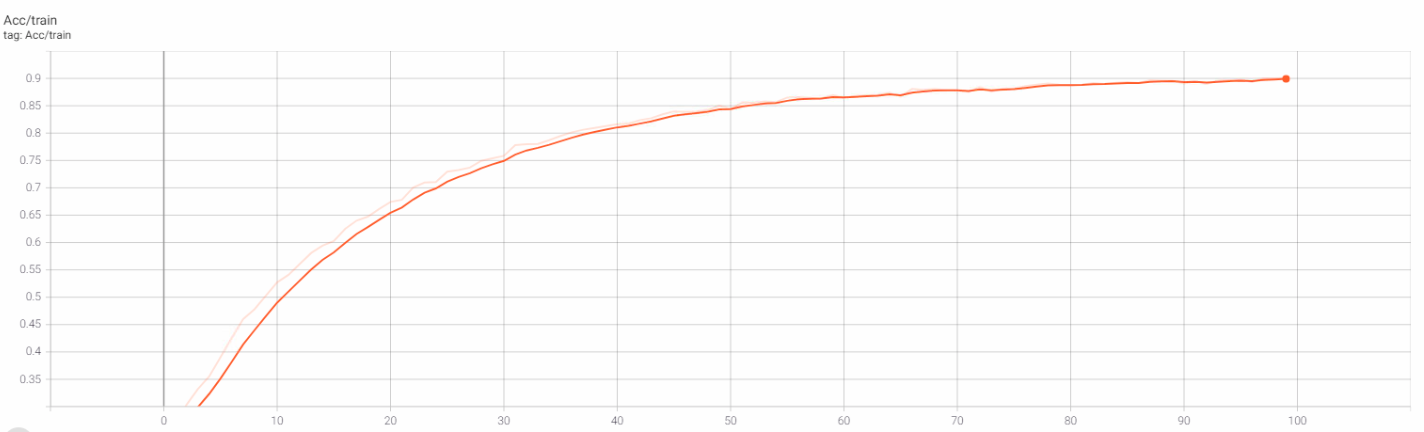
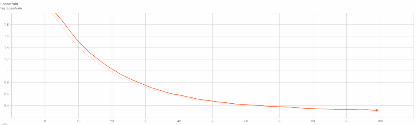
Chúng ta sẽ tiến hành huấn luyện model với 100 epochs:
num_epochs=100
training(myModel, train_dl, num_epochs)
Sau 100 epochs, chúng ta thu được kết quả:
Epoch: 0, Loss: 2.22, Accuracy: 0.19
Epoch: 1, Loss: 2.10, Accuracy: 0.27
...
Epoch: 98, Loss: 0.31, Accuracy: 0.90
Epoch: 99, Loss: 0.31, Accuracy: 0.90
Finished Training
Và đồ thị Training Loss, Training Acc trên Tensorboard:
6. Inference
Tiếp theo, chúng ta sử dụng model đã lưu đề tiến hành dự đoán và đánh giá độ chính xác trên tập Test.
# ----------------------------
# Inference
# ----------------------------
def inference (model, test_dl):
    correct_prediction = 0
    total_prediction = 0

    # Disable gradient updates
    with torch.no_grad():
        for data in test_dl:
            # Get the input features and target labels, and put them on the GPU
            inputs, labels = data[0].to(device), data[1].to(device)

            # Normalize the inputs
            inputs_m, inputs_s = inputs.mean(), inputs.std()
            inputs = (inputs - inputs_m) / inputs_s

            # Get predictions
            outputs = model(inputs)

            # Get the predicted class with the highest score
            _, prediction = torch.max(outputs,1)
            # Count of predictions that matched the target label
            correct_prediction += (prediction == labels).sum().item()
            total_prediction += prediction.shape[0]

    acc = correct_prediction/total_prediction
    print(f'Accuracy: {acc:.2f}, Total items: {total_prediction}')

# Run inference on trained model with the validation set load best model weights
model_inf = nn.DataParallel(AudioClassifier())
device = torch.device("cuda" if torch.cuda.is_available() else "cpu")
model_inf = model_inf.to(device)
model_inf.load_state_dict(torch.load('model.pt'))
model_inf.eval()

inference(model_inf, val_dl)
Kết quả:
Accuracy: 0.90, Total items: 1746
Trên tập Test, độ chính xác vẫn đạt đuọc 90%. Điều này chứng tỏ model của chúng ta hoạt động khá tốt, không bị hiện tượng Overfitting.
7. Hướng mở rộng
Kết quả đạt được của chúng ta đã khá tốt rồi, tuy nhiên vẫn còn một số hướng có khả năng sẽ làm cho kết quả tốt hơn. Nếu gặp bài toán Audio Classification trong thực tế, bạn có thể thử áp dụng những cách này xem độ chính xác của model có được cải thiện thêm không nhế.
7.1 Thay thế kiến trúc CNN model khác
Ở đây, chúng ta đang tự xây dựng kiến trúc CNN model. Như bạn đã biết, có khá nhiều kiến trúc CNN model kinh điển cho bài toán Image Classification như VGG, ResNet, InceptionNet, … Hãy thử với các kiến trúc này hoặc huấn luyện từ đầu hoặc sử dụng Transfer Learing …
7.2 Thay đổi Audio Features
Như bài trước đã phân tích, Audio Features có thể ở dạng Mel Spectrogram hoặc MFCCs. Bài này chúng ta đã sử dụng Mel Spectrogram rồi, còn lại MFCC là dành cho các bạn thử.
7.3 Mel Spectrogram Hyper-parameters Tuning
Để tạo ra Mel Spectrogram, chúng ta cần cung cấp một số Hyper-parameters. Giá trị của các Hyper-parameters này ảnh hưởng ít nhiều đến Mel Spectrogram được tạo ra, từ đó ảnh hưởng đến kết quả của model. Hãy thử Tune các Hyper-parameters của Mel Spectrogram xem sao nhé. Tham khảo thêm tại đây.
7.4 Áp dụng phương pháp k-Fold Cross Validation
k-Fold Cross Validation vẫn là một trong những phương pháp khá hiệu quả đổi với các bài toán có sự mất cân bằng về dữ liệu. Dataset sử dụng trong bài này cũng được phân ra thành 10 folds, ngụ ý rằng nên sử dụng phương pháp k-Fold Cross Validation đối với nó để có được kết quả tốt hơn. Code cho phương pháp này mình cũng đã viết nhưng chưa có thời gian chạy thử để so sánh.
8. Kết luận
Bài thứ tư trong chuỗi các bài viết về Audio Deep Learning này, chúng ta đã cùng nhau thực hiện code hoàn chỉnh bài toán Audio Classification. Một số hướng tiếp cận mở rộng cũng được đưa ra để các bạn nghiên cứu thêm.
Source code bài này mình để ở đây.
Trong bài thứ 5 tiếp theo, chúng ta sẽ thảo luận về bài toán Speech Recognition. Mời các bạn đón đọc.
9. Tham khảo
[1] Ketan Doshi, “Audio Deep Learning Made Simple (Part 3): Data Preparation and Augmentation”, Available online: https://towardsdatascience.com/audio-deep-learning-made-simple-sound-classification-step-by-step-cebc936bbe5 (Accessed on 05 Jun 2021).
[2] Scott Duda, “Urban Environmental Audio Classification Using Mel Spectrograms”, Available online: https://scottmduda.medium.com/urban-environmental-audio-classification-using-mel-spectrograms-706ee6f8dcc1 (Accessed on 05 Jun 2021).