DP4ML - Feature Selection - Phần 4 - Select Features for Numerical Output
Bài thứ 11 trong chuỗi các bài viết về chủ đề Data Preparation cho các mô hình ML và là bài thứ 4 về Feature Selection. Trong bài này, chúng ta sẽ tìm hiểu phương pháp lựa chọn features đối với dữ liệu có Ouput Variance thuộc kiểu Numberical thông qua việc thực hành trên một bộ dữ liệu giả được sinh ra ngẫu nhiên.
1. Regression Dataset
Chúng ta sẽ sử dụng tập dữ liệu Regresion (tức dữ liệu có Ouput Variance ở dạng Numerical) làm cơ sở của bài thực hành này. Nhớ lại rằng một bài toán hồi quy là một bài toán mà chúng ta muốn dự đoán một giá trị số cụ thể. Trong trường hợp này, chúng ta cũng sẽ tạo ra một tập dữ liệu mà các Input Variables cũng có dạng Numerical. Hàm make regression() từ thư viện scikit-learn có thể được sử dụng để định nghĩa một tập dữ liệu như vậy. Nó cung cấp khả năng kiểm soát số lượng mẫu, số lượng các Input Variables và quan trọng là số lượng các Input Variables đó có liên quan và không liên quan đến Output Variable. Điều này rất quan trọng vì chúng ta đặc biệt mong muốn một tập dữ liệu mà chúng ta biết trước có một số Input Variables không liên quan đến Output Variable. Cụ thể ở bài này, mình sẽ tạo ra một tập dữ liệu với 1.000 mẫu, mỗi mẫu có 100 Input Variables, trong đó 10 mẫu là thông tin liên quan và 90 mẫu còn lại là không liên quan đến Output Variable.
...
# generate regression dataset
X, y = make_regression(n_samples=1000, n_features=100, n_informative=10, noise=0.1, random_state=1)
Chúng ta hy vọng là các kỹ thuật Feature Selection có thể xác định đúng hoặc gần đúng các Input Variables có liên quan đến Output Variable như chúng ta đã định nghĩa từ đầu. Sau khi được xác định điều đó, chúng ta có thể tiến hành chia dữ liệu thành các train/test để tạo ra mô hình dự đoán.
# load and summarize the dataset
from sklearn.datasets import make_regression
from sklearn.model_selection import train_test_split
# generate regression dataset
X, y = make_regression(n_samples=1000, n_features=100, n_informative=10, noise=0.1, random_state=1)
# split into train and test sets
X_train, X_test, y_train, y_test = train_test_split(X, y, test_size=0.33, random_state=1)
# summarize
print('Train', X_train.shape, y_train.shape)
print('Test', X_test.shape, y_test.shape)
Kết quả thực hiện:
Train (670, 100) (670,)
Test (330, 100) (330,)
2. Numerical Feature Selection
Có 2 kỹ thuật Feature Selection phổ biến có thể sử dụng cho Numerical Input/Output Variables, đó là Correlation Statistic và Mutual Information.
2.1 Correlation Statistic
Correlation (sự tương quan) là thước đo mức độ thay đổi của hai biến số cùng nhau. Có lẽ thước đo Correlation phổ biến nhất là Pearson’s Correlation. Nó giả định phân phối Gauss cho mỗi biến và báo cáo về mối quan hệ tuyến tính của chúng.
Điểm tương quan tuyến tính thường là một giá trị từ -1 đến 1 với 0 thể hiện không có mối quan hệ nào. Đối với việc lựa chọn Input Variables, chúng ta thường quan tâm đến giá trị dương càng lớn càng tốt, bởi vì đó mối quan hệ càng lớn và nhiều khả năng Input Variable đó nên được chọn để huấn luyện mô hình. Như vậy, mối tương quan tuyến tính có thể được chuyển đổi thành một thống kê tương quan chỉ với các giá trị dương.
Correlation Statistic được implement trong scikit-learn bằng hàm f_regression(). Cách sử dụng nó tương tự như các bài trước.
# example of correlation feature selection for numerical data
from sklearn.datasets import make_regression
from sklearn.model_selection import train_test_split
from sklearn.feature_selection import SelectKBest
from sklearn.feature_selection import f_regression
from matplotlib import pyplot

# feature selection
def select_features(X_train, y_train, X_test):
	# configure to select all features
	fs = SelectKBest(score_func=f_regression, k='all')
	# learn relationship from training data
	fs.fit(X_train, y_train)
	# transform train input data
	X_train_fs = fs.transform(X_train)
	# transform test input data
	X_test_fs = fs.transform(X_test)
	return X_train_fs, X_test_fs, fs

# load the dataset
X, y = make_regression(n_samples=1000, n_features=100, n_informative=10, noise=0.1, random_state=1)
# split into train and test sets
X_train, X_test, y_train, y_test = train_test_split(X, y, test_size=0.33, random_state=1)
# feature selection
X_train_fs, X_test_fs, fs = select_features(X_train, y_train, X_test)
# what are scores for the features
for i in range(len(fs.scores_)):
	print('Feature %d: %f' % (i, fs.scores_[i]))
# plot the scores
pyplot.bar([i for i in range(len(fs.scores_))], fs.scores_)
pyplot.show()
Kết quả thực hiện:
Feature 0: 0.009419
Feature 1: 1.018881
Feature 2: 1.205187
Feature 3: 0.000138
Feature 4: 0.167511
Feature 5: 5.985083
Feature 6: 0.062405
Feature 7: 1.455257
Feature 8: 0.420384
Feature 9: 101.392225
Feature 10: 0.387091
Feature 11: 1.581124
Feature 12: 3.014463
Feature 13: 0.232705
Feature 14: 0.076281
Feature 15: 4.299652
Feature 16: 1.497530
Feature 17: 0.261242
Feature 18: 5.960005
Feature 19: 0.523219
Feature 20: 0.003365
Feature 21: 0.024178
Feature 22: 0.220958
Feature 23: 0.576770
Feature 24: 0.627198
Feature 25: 0.350687
Feature 26: 0.281877
Feature 27: 0.584210
Feature 28: 52.196337
Feature 29: 0.046855
Feature 30: 0.147323
Feature 31: 0.368485
Feature 32: 0.077631
Feature 33: 0.698140
Feature 34: 45.744046
Feature 35: 2.047376
Feature 36: 0.786270
Feature 37: 0.996190
Feature 38: 2.733533
Feature 39: 63.957656
Feature 40: 231.885540
Feature 41: 1.372448
Feature 42: 0.581860
Feature 43: 1.072930
Feature 44: 1.066976
Feature 45: 0.344656
Feature 46: 13.951551
Feature 47: 3.575080
Feature 48: 0.007299
Feature 49: 0.004651
Feature 50: 1.094585
Feature 51: 0.241065
Feature 52: 0.355137
Feature 53: 0.020294
Feature 54: 0.154567
Feature 55: 2.592512
Feature 56: 0.300175
Feature 57: 0.357798
Feature 58: 3.060090
Feature 59: 0.890357
Feature 60: 122.132164
Feature 61: 2.029982
Feature 62: 0.091551
Feature 63: 1.081123
Feature 64: 0.056041
Feature 65: 2.930717
Feature 66: 0.054886
Feature 67: 1.332787
Feature 68: 0.145579
Feature 69: 0.986331
Feature 70: 0.092661
Feature 71: 0.083219
Feature 72: 0.198847
Feature 73: 2.065792
Feature 74: 0.236594
Feature 75: 0.512608
Feature 76: 1.095650
Feature 77: 0.015359
Feature 78: 2.193730
Feature 79: 1.574530
Feature 80: 5.360863
Feature 81: 0.041874
Feature 82: 5.717705
Feature 83: 0.436560
Feature 84: 5.594438
Feature 85: 0.000065
Feature 86: 0.026748
Feature 87: 0.408422
Feature 88: 2.092557
Feature 89: 9.568498
Feature 90: 0.642445
Feature 91: 0.065794
Feature 92: 198.705931
Feature 93: 0.073807
Feature 94: 1.048605
Feature 95: 0.004106
Feature 96: 0.042110
Feature 97: 0.034228
Feature 98: 0.792433
Feature 99: 0.015365
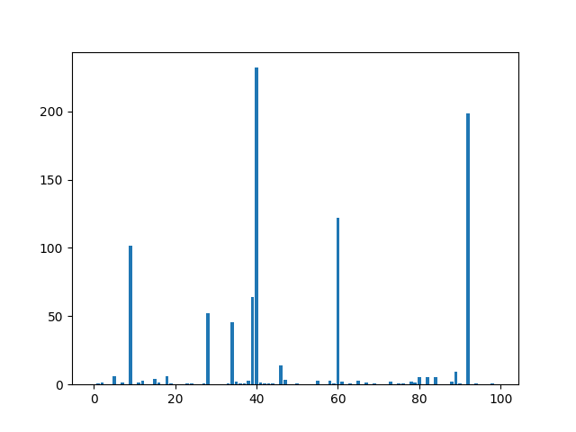
Correlation Score của mỗi features và target được tính toán và hiển thị lên đồ thị. Quan sát ta thấy, có khoảng 8 đến 10 features là có mức đó liên quan nhiều nhất đến target. Set k=10 khi sử dụng Correlation Statistic với SelectKBest().
2.2 Mutual Information Feature Selection
Vẫn lại là Mutual Information, nó vẫn được sử dụng ở đây. Tuy nhiên, khác với các lần trước là bài toán Binary Classification (sử dụng hàm mutual_info_classif) thì lần này là bài toán Regression nên hàm implement của Mutual Information là mutual_info_regression.
# example of mutual information feature selection for numerical input data
from sklearn.datasets import make_regression
from sklearn.model_selection import train_test_split
from sklearn.feature_selection import SelectKBest
from sklearn.feature_selection import mutual_info_regression
from matplotlib import pyplot

# feature selection
def select_features(X_train, y_train, X_test):
	# configure to select all features
	fs = SelectKBest(score_func=mutual_info_regression, k='all')
	# learn relationship from training data
	fs.fit(X_train, y_train)
	# transform train input data
	X_train_fs = fs.transform(X_train)
	# transform test input data
	X_test_fs = fs.transform(X_test)
	return X_train_fs, X_test_fs, fs

# load the dataset
X, y = make_regression(n_samples=1000, n_features=100, n_informative=10, noise=0.1, random_state=1)
# split into train and test sets
X_train, X_test, y_train, y_test = train_test_split(X, y, test_size=0.33, random_state=1)
# feature selection
X_train_fs, X_test_fs, fs = select_features(X_train, y_train, X_test)
# what are scores for the features
for i in range(len(fs.scores_)):
	print('Feature %d: %f' % (i, fs.scores_[i]))
# plot the scores
pyplot.bar([i for i in range(len(fs.scores_))], fs.scores_)
pyplot.show()
Kết quả thực hiện:
Feature 0: 0.045484
Feature 1: 0.000000
Feature 2: 0.000000
Feature 3: 0.000000
Feature 4: 0.024816
Feature 5: 0.000000
Feature 6: 0.022659
Feature 7: 0.000000
Feature 8: 0.000000
Feature 9: 0.074320
Feature 10: 0.000000
Feature 11: 0.000000
Feature 12: 0.000000
Feature 13: 0.000000
Feature 14: 0.020390
Feature 15: 0.004307
Feature 16: 0.000000
Feature 17: 0.000000
Feature 18: 0.016566
Feature 19: 0.003688
Feature 20: 0.007579
Feature 21: 0.018640
Feature 22: 0.025206
Feature 23: 0.017967
Feature 24: 0.069173
Feature 25: 0.000000
Feature 26: 0.022232
Feature 27: 0.000000
Feature 28: 0.007849
Feature 29: 0.012849
Feature 30: 0.017402
Feature 31: 0.008083
Feature 32: 0.047321
Feature 33: 0.002829
Feature 34: 0.028968
Feature 35: 0.000000
Feature 36: 0.071652
Feature 37: 0.027969
Feature 38: 0.000000
Feature 39: 0.064796
Feature 40: 0.137695
Feature 41: 0.008732
Feature 42: 0.003983
Feature 43: 0.000000
Feature 44: 0.009387
Feature 45: 0.000000
Feature 46: 0.038385
Feature 47: 0.000000
Feature 48: 0.000000
Feature 49: 0.000000
Feature 50: 0.000000
Feature 51: 0.000000
Feature 52: 0.000000
Feature 53: 0.008130
Feature 54: 0.041779
Feature 55: 0.000000
Feature 56: 0.000000
Feature 57: 0.000000
Feature 58: 0.031228
Feature 59: 0.002689
Feature 60: 0.146192
Feature 61: 0.000000
Feature 62: 0.000000
Feature 63: 0.000000
Feature 64: 0.018194
Feature 65: 0.021368
Feature 66: 0.046071
Feature 67: 0.034707
Feature 68: 0.033530
Feature 69: 0.002262
Feature 70: 0.018332
Feature 71: 0.000000
Feature 72: 0.000000
Feature 73: 0.074876
Feature 74: 0.000000
Feature 75: 0.004429
Feature 76: 0.002617
Feature 77: 0.031354
Feature 78: 0.000000
Feature 79: 0.000000
Feature 80: 0.000000
Feature 81: 0.033931
Feature 82: 0.010400
Feature 83: 0.019373
Feature 84: 0.000000
Feature 85: 0.033191
Feature 86: 0.000000
Feature 87: 0.028745
Feature 88: 0.000000
Feature 89: 0.000000
Feature 90: 0.000000
Feature 91: 0.017698
Feature 92: 0.129797
Feature 93: 0.000000
Feature 94: 0.002171
Feature 95: 0.029995
Feature 96: 0.000000
Feature 97: 0.014428
Feature 98: 0.000000
Feature 99: 0.000000

Trong trường hợp này thì số lượng features có sự liên quan nhiều đến target lớn hơn con số 10. Điều này có lẽ do ảnh hưởng của nhiễu mà ta thêm vào khi tạo dữ liệu.
3. Modeling With Selected Features
3.1 Base model
Base model được xây dựng với tất cả dữ liệu mặc định.
# evaluation of a model using all input features
from sklearn.datasets import make_regression
from sklearn.model_selection import train_test_split
from sklearn.linear_model import LinearRegression
from sklearn.metrics import mean_absolute_error
# load the dataset
X, y = make_regression(n_samples=1000, n_features=100, n_informative=10, noise=0.1, random_state=1)
# split into train and test sets
X_train, X_test, y_train, y_test = train_test_split(X, y, test_size=0.33, random_state=1)
# fit the model
model = LinearRegression()
model.fit(X_train, y_train)
# evaluate the model
yhat = model.predict(X_test)
# evaluate predictions
mae = mean_absolute_error(y_test, yhat)
print('MAE: %.3f' % mae)
Kết quả thực hiện:
MAE: 0.086
3.2 Model Built Using Correlation Features
# evaluation of a model using 10 features chosen with correlation
from sklearn.datasets import make_regression
from sklearn.model_selection import train_test_split
from sklearn.feature_selection import SelectKBest
from sklearn.feature_selection import f_regression
from sklearn.linear_model import LinearRegression
from sklearn.metrics import mean_absolute_error

# feature selection
def select_features(X_train, y_train, X_test):
	# configure to select a subset of features
	fs = SelectKBest(score_func=f_regression, k=10)
	# learn relationship from training data
	fs.fit(X_train, y_train)
	# transform train input data
	X_train_fs = fs.transform(X_train)
	# transform test input data
	X_test_fs = fs.transform(X_test)
	return X_train_fs, X_test_fs, fs

# load the dataset
X, y = make_regression(n_samples=1000, n_features=100, n_informative=10, noise=0.1, random_state=1)
# split into train and test sets
X_train, X_test, y_train, y_test = train_test_split(X, y, test_size=0.33, random_state=1)
# feature selection
X_train_fs, X_test_fs, fs = select_features(X_train, y_train, X_test)
# fit the model
model = LinearRegression()
model.fit(X_train_fs, y_train)
# evaluate the model
yhat = model.predict(X_test_fs)
# evaluate predictions
mae = mean_absolute_error(y_test, yhat)
print('MAE: %.3f' % mae)
Kết quả thực hiện:
MAE: 2.74
Trong trường hợp này, chúng ta thấy rằng mô hình đạt được MAE khoảng 2.7, lớn hơn nhiều so với Base model (0.086). Mặc dù đã nhận ra được các features nào là quan trọng cần chọn, nhưng việc xây dựng một mô hình từ những features này lại không tạo ra một mô hình có kết quả tốt hơn. Điều này có thể là do các features quan trọng đối với mục tiêu đã bị bỏ qua, có nghĩa là phương pháp Correlation Statistic đang bị đánh lừa về những gì là quan trọng khi lựa chọn features.
Chúng ta sẽ thử lại bằng cách tăng số lượng features được lựa chọn lên thành 90. Kết quả thu được MAE = 0.085, tốt hơn một chút so với Base model.
3.3 Model Built Using Mutual Information Features
# evaluation of a model using 88 features chosen with mutual information
from sklearn.datasets import make_regression
from sklearn.model_selection import train_test_split
from sklearn.feature_selection import SelectKBest
from sklearn.feature_selection import mutual_info_regression
from sklearn.linear_model import LinearRegression
from sklearn.metrics import mean_absolute_error

# feature selection
def select_features(X_train, y_train, X_test):
	# configure to select a subset of features
	fs = SelectKBest(score_func=mutual_info_regression, k=88)
	# learn relationship from training data
	fs.fit(X_train, y_train)
	# transform train input data
	X_train_fs = fs.transform(X_train)
	# transform test input data
	X_test_fs = fs.transform(X_test)
	return X_train_fs, X_test_fs, fs

# load the dataset
X, y = make_regression(n_samples=1000, n_features=100, n_informative=10, noise=0.1, random_state=1)
# split into train and test sets
X_train, X_test, y_train, y_test = train_test_split(X, y, test_size=0.33, random_state=1)
# feature selection
X_train_fs, X_test_fs, fs = select_features(X_train, y_train, X_test)
# fit the model
model = LinearRegression()
model.fit(X_train_fs, y_train)
# evaluate the model
yhat = model.predict(X_test_fs)
# evaluate predictions
mae = mean_absolute_error(y_test, yhat)
print('MAE: %.3f' % mae)
Kết quả thực hiện:
MAE: 0.084
Model lần này có kết quả tốt hơn hai lần trước một chút, vẫn lựa chọn 88 features.
3.4 Tune the Number of Selected Features
Biết được rằng Mutual Information cho kết quả tốt nhất rồi. Ta tiếp tục thử xem liệu có giá nào của k để thu được model tốt hơn nữa không bằng cách thực thiện tune giá trị của k. Lần này chúng ta sẽ sử dụng metric neg_mean_absolute_error để đánh giá.
# compare different numbers of features selected using mutual information
from sklearn.datasets import make_regression
from sklearn.model_selection import RepeatedKFold
from sklearn.feature_selection import SelectKBest
from sklearn.feature_selection import mutual_info_regression
from sklearn.linear_model import LinearRegression
from sklearn.pipeline import Pipeline
from sklearn.model_selection import GridSearchCV
# define dataset
X, y = make_regression(n_samples=1000, n_features=100, n_informative=10, noise=0.1, random_state=1)
# define the evaluation method
cv = RepeatedKFold(n_splits=10, n_repeats=3, random_state=1)
# define the pipeline to evaluate
model = LinearRegression()
fs = SelectKBest(score_func=mutual_info_regression)
pipeline = Pipeline(steps=[('sel',fs), ('lr', model)])
# define the grid
grid = dict()
grid['sel__k'] = [i for i in range(X.shape[1]-20, X.shape[1]+1)]
# define the grid search
search = GridSearchCV(pipeline, grid, scoring='neg_mean_absolute_error', n_jobs=-1, cv=cv)
# perform the search
results = search.fit(X, y)
# summarize best
print('Best MAE: %.3f' % results.best_score_)
print('Best Config: %s' % results.best_params_)
# summarize all
means = results.cv_results_['mean_test_score']
params = results.cv_results_['params']
for mean, param in zip(means, params):
    print('>%.3f with: %r' % (mean, param))
Kết quả thực hiện:
Best MAE: -0.082
Best Config: {'sel__k': 81}
>-1.100 with: {'sel__k': 80}
>-0.082 with: {'sel__k': 81}
>-0.082 with: {'sel__k': 82}
>-0.082 with: {'sel__k': 83}
>-0.082 with: {'sel__k': 84}
>-0.082 with: {'sel__k': 85}
>-0.082 with: {'sel__k': 86}
>-0.082 with: {'sel__k': 87}
>-0.082 with: {'sel__k': 88}
>-0.083 with: {'sel__k': 89}
>-0.083 with: {'sel__k': 90}
>-0.083 with: {'sel__k': 91}
>-0.083 with: {'sel__k': 92}
>-0.083 with: {'sel__k': 93}
>-0.083 with: {'sel__k': 94}
>-0.083 with: {'sel__k': 95}
>-0.083 with: {'sel__k': 96}
>-0.083 with: {'sel__k': 97}
>-0.083 with: {'sel__k': 98}
>-0.083 with: {'sel__k': 99}
>-0.083 with: {'sel__k': 100}
Rất may là ta đã đi đúng hướng, không lãng phí thời gian vì ta đã tìm được model tốt hơn, MAE=0.082 với k=81.
Cuối cùng, nếu muốn xem cụ thể giá trị MAE là bao nhiêu đối với từng giá trị của k, ta code như sau:
# compare different numbers of features selected using mutual information
from numpy import mean
from numpy import std
from sklearn.datasets import make_regression
from sklearn.model_selection import cross_val_score
from sklearn.model_selection import RepeatedKFold
from sklearn.feature_selection import SelectKBest
from sklearn.feature_selection import mutual_info_regression
from sklearn.linear_model import LinearRegression
from sklearn.pipeline import Pipeline
from matplotlib import pyplot
# define dataset
X, y = make_regression(n_samples=1000, n_features=100, n_informative=10, noise=0.1, random_state=1)
# define number of features to evaluate
num_features = [i for i in range(X.shape[1]-19, X.shape[1]+1)]
# enumerate each number of features
results = list()
for k in num_features:
	# create pipeline
	model = LinearRegression()
	fs = SelectKBest(score_func=mutual_info_regression, k=k)
	pipeline = Pipeline(steps=[('sel',fs), ('lr', model)])
	# evaluate the model
	cv = RepeatedKFold(n_splits=10, n_repeats=3, random_state=1)
	scores = cross_val_score(pipeline, X, y, scoring='neg_mean_absolute_error', cv=cv, n_jobs=-1)
	results.append(scores)
	# summarize the results
	print('>%d %.3f (%.3f)' % (k, mean(scores), std(scores)))
# plot model performance for comparison
pyplot.boxplot(results, labels=num_features, showmeans=True)
pyplot.show()
Kết quả thực hiện:
>81 -0.082 (0.006)
>82 -0.082 (0.006)
>83 -0.082 (0.006)
>84 -0.082 (0.006)
>85 -0.082 (0.006)
>86 -0.082 (0.006)
>87 -0.082 (0.006)
>88 -0.082 (0.006)
>89 -0.083 (0.006)
>90 -0.083 (0.006)
>91 -0.083 (0.006)
>92 -0.083 (0.006)
>93 -0.083 (0.006)
>94 -0.083 (0.006)
>95 -0.083 (0.006)
>96 -0.083 (0.006)
>97 -0.083 (0.006)
>98 -0.083 (0.006)
>99 -0.083 (0.006)
>100 -0.083 (0.006)
4. Kết luận
Bài thứ 4 về chủ đề Feature Selection, mình đã giới thiệu 2 kỹ thuật Correlation Statistic t và Mutual Information áp dụng cho Input/Output Variables dạng Numerical. Toàn bộ code của bài này, các bạn có thể tham khảo tại đây.
Bài tiếp theo sẽ là cách sử dụng thuật toán Recursive Feature Elimination (RFE) trong việc Feature Selection. Mời các bạn đón đọc.
5. Tham khảo
[1] Jason Brownlee, “Data Preparation for Machine Learning”, Book: https://machinelearningmastery.com/data-preparation-for-machine-learning/.