SuNT's Blog | AI in Practical

Bài thứ 10 trong chuỗi các bài viết về chủ đề Data Preparation cho các mô hình ML và là bài thứ 3 về Feature Selection. Trong bài này, chúng ta sẽ tìm hiểu phương pháp lựa chọn features đối với dữ liệu có Input Variance thuộc kiểu Numberical thông qua việc thực hành trên một bộ dữ liệu cụ thể.

1. Pima Indians Dataset

Pima Indians Dataset là bộ dữ liệu đã được chúng ta sử dụng trước đó trong bài thứ 4 về DP4ML. Trong bài này, chúng ta tiếp tục sử dụng nó.

Code đọc và chuẩn bị dữ liệu như sau:

# load and summarize the dataset
from pandas import read_csv
from sklearn.model_selection import train_test_split

# load the dataset
def load_dataset(filename):
	# load the dataset as a pandas DataFrame
	data = read_csv(filename, header=None)
	# retrieve numpy array
	dataset = data.values
	# split into input (X) and output (y) variables
	X = dataset[:, :-1]
	y = dataset[:,-1]
	return X, y

# load the dataset
X, y = load_dataset('pima-indians-diabetes.csv')
# split into train and test sets
X_train, X_test, y_train, y_test = train_test_split(X, y, test_size=0.33, random_state=1)
# summarize
print('Train', X_train.shape, y_train.shape)
print('Test', X_test.shape, y_test.shape)

Vì các Input/Output Variables đều đã ở dạng Numerical nên chúng ta không cần thực hiện Transform Data nữa.

2. Numerical Feature Selection

Hai kỹ thuật có thể áp dụng cho Input Variables dạng Numerical để thực hiện Feature Selection là: ANOVE F-Statistic và Mutual Information Statistic.

2.1 ANOVA F-Test (Statistic)

ANOVA - Analysis Of Variance, là một bài kiểm tra giả thuyết thống kê tham số để xác định xem các giá trị trung bình của hai hoặc nhiều mẫu dữ liệu có cùng phân phối với nhau hay không. F-Statistic, hay F-test, là một loại kiểm tra thống kê tính toán tỷ lệ giữa các giá trị phương sai, chẳng hạn như phương sai từ hai mẫu khác nhau. Phương pháp ANOVA là một loại F-Statistic, được gọi ở đây là ANOVA F-Test.

Điều quan trọng, ANOVA được sử dụng khi một biến là số và một biến là Categorical, chẳng hạn như biến đầu vào số và biến mục tiêu phân loại trong nhiệm vụ phân loại. Kết quả của thử nghiệm này có thể được sử dụng để lựa chọn features bằng cách loại bỏ những features độc lập với Output Variables khỏi tập dữ liệu.

Tương tự như Chi-Squared và Mutual Information ở bài trước, ANOVA F-Test cũng được implement trong Scikit-learn bởi hàm f-classif().

# example of anova f-test feature selection for numerical data
from pandas import read_csv
from sklearn.model_selection import train_test_split
from sklearn.feature_selection import SelectKBest
from sklearn.feature_selection import f_classif
from matplotlib import pyplot

# load the dataset
def load_dataset(filename):
	# load the dataset as a pandas DataFrame
	data = read_csv(filename, header=None)
	# retrieve numpy array
	dataset = data.values
	# split into input (X) and output (y) variables
	X = dataset[:, :-1]
	y = dataset[:,-1]
	return X, y

# feature selection
def select_features(X_train, y_train, X_test):
	# configure to select all features
	fs = SelectKBest(score_func=f_classif, k='all')
	# learn relationship from training data
	fs.fit(X_train, y_train)
	# transform train input data
	X_train_fs = fs.transform(X_train)
	# transform test input data
	X_test_fs = fs.transform(X_test)
	return X_train_fs, X_test_fs, fs

# load the dataset
X, y = load_dataset('pima-indians-diabetes.csv')
# split into train and test sets
X_train, X_test, y_train, y_test = train_test_split(X, y, test_size=0.33, random_state=1)
# feature selection
X_train_fs, X_test_fs, fs = select_features(X_train, y_train, X_test)
# what are scores for the features
for i in range(len(fs.scores_)):
	print('Feature %d: %f' % (i, fs.scores_[i]))
# plot the scores
pyplot.bar([i for i in range(len(fs.scores_))], fs.scores_)
pyplot.show()

Kết quả thực hiện:

Feature 0: 16.527385
Feature 1: 131.325562
Feature 2: 0.042371
Feature 3: 1.415216
Feature 4: 12.778966
Feature 5: 49.209523
Feature 6: 13.377142
Feature 7: 25.126440

Nhìn vào đây, ta có thể chọn k=6 khi sử dụng kỹ thuật này.

2.2 Mutual Information Feature Selection

Kỹ thuật này mình đã giới thiệu ở bài số 9. Cách sử dụng nó cho Input Variables dạng Numerical cũng không có gì thay đổi.

# example of mutual information feature selection for numerical input data
from pandas import read_csv
from sklearn.model_selection import train_test_split
from sklearn.feature_selection import SelectKBest
from sklearn.feature_selection import mutual_info_classif
from matplotlib import pyplot

# load the dataset
def load_dataset(filename):
	# load the dataset as a pandas DataFrame
	data = read_csv(filename, header=None)
	# retrieve numpy array
	dataset = data.values
	# split into input (X) and output (y) variables
	X = dataset[:, :-1]
	y = dataset[:,-1]
	return X, y

# feature selection
def select_features(X_train, y_train, X_test):
	# configure to select all features
	fs = SelectKBest(score_func=mutual_info_classif, k='all')
	# learn relationship from training data
	fs.fit(X_train, y_train)
	# transform train input data
	X_train_fs = fs.transform(X_train)
	# transform test input data
	X_test_fs = fs.transform(X_test)
	return X_train_fs, X_test_fs, fs

# load the dataset
X, y = load_dataset('pima-indians-diabetes.csv')
# split into train and test sets
X_train, X_test, y_train, y_test = train_test_split(X, y, test_size=0.33, random_state=1)
# feature selection
X_train_fs, X_test_fs, fs = select_features(X_train, y_train, X_test)
# what are scores for the features
for i in range(len(fs.scores_)):
	print('Feature %d: %f' % (i, fs.scores_[i]))
# plot the scores
pyplot.bar([i for i in range(len(fs.scores_))], fs.scores_)
pyplot.show()

Kết quả:

Feature 0: 0.000000
Feature 1: 0.120654
Feature 2: 0.022504
Feature 3: 0.027918
Feature 4: 0.031081
Feature 5: 0.073868
Feature 6: 0.019561
Feature 7: 0.030316

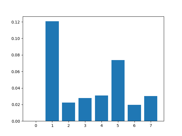
Căn cứ vào đây thì có lẽ k=2 hoặc k=3 sẽ là lựa chọn phù hợp.

3. Modeling With Selected Features

Vẫn lựa chọn thuật toán Logistic Regression để thực hiện mô hình hóa tập dữ liệu Pima Indians với các kỹ thuật Feature Selection bên trên.

3.1 Base model

Base model được xây dựng với tất cả dữ liệu mặc định.

# evaluation of a model using all input features
from pandas import read_csv
from sklearn.model_selection import train_test_split
from sklearn.linear_model import LogisticRegression
from sklearn.metrics import accuracy_score

# load the dataset
def load_dataset(filename):
	# load the dataset as a pandas DataFrame
	data = read_csv(filename, header=None)
	# retrieve numpy array
	dataset = data.values
	# split into input (X) and output (y) variables
	X = dataset[:, :-1]
	y = dataset[:,-1]
	return X, y

# load the dataset
X, y = load_dataset('pima-indians-diabetes.csv')
# split into train and test sets
X_train, X_test, y_train, y_test = train_test_split(X, y, test_size=0.33, random_state=1)
# fit the model
model = LogisticRegression(solver='liblinear')
model.fit(X_train, y_train)
# evaluate the model
yhat = model.predict(X_test)
# evaluate predictions
accuracy = accuracy_score(y_test, yhat)
print('Accuracy: %.2f' % (accuracy*100))

Kết quả:

Accuracy: 77.56

3.2 Model Built Using ANOVA F-test Features

# evaluation of a model using 4 features chosen with anova f-test
from pandas import read_csv
from sklearn.model_selection import train_test_split
from sklearn.feature_selection import SelectKBest
from sklearn.feature_selection import f_classif
from sklearn.linear_model import LogisticRegression
from sklearn.metrics import accuracy_score

# load the dataset
def load_dataset(filename):
	# load the dataset as a pandas DataFrame
	data = read_csv(filename, header=None)
	# retrieve numpy array
	dataset = data.values
	# split into input (X) and output (y) variables
	X = dataset[:, :-1]
	y = dataset[:,-1]
	return X, y

# feature selection
def select_features(X_train, y_train, X_test):
	# configure to select a subset of features
	fs = SelectKBest(score_func=f_classif, k=4)
	# learn relationship from training data
	fs.fit(X_train, y_train)
	# transform train input data
	X_train_fs = fs.transform(X_train)
	# transform test input data
	X_test_fs = fs.transform(X_test)
	return X_train_fs, X_test_fs, fs

# load the dataset
X, y = load_dataset('pima-indians-diabetes.csv')
# split into train and test sets
X_train, X_test, y_train, y_test = train_test_split(X, y, test_size=0.33, random_state=1)
# feature selection
X_train_fs, X_test_fs, fs = select_features(X_train, y_train, X_test)
# fit the model
model = LogisticRegression(solver='liblinear')
model.fit(X_train_fs, y_train)
# evaluate the model
yhat = model.predict(X_test_fs)
# evaluate predictions
accuracy = accuracy_score(y_test, yhat)
print('Accuracy: %.2f' % (accuracy*100))

Kết quả:

Accuracy: 78.74

3.3 Model Built Using Mutual Information Features

# evaluation of a model using 4 features chosen with mutual information
from pandas import read_csv
from sklearn.model_selection import train_test_split
from sklearn.feature_selection import SelectKBest
from sklearn.feature_selection import mutual_info_classif
from sklearn.linear_model import LogisticRegression
from sklearn.metrics import accuracy_score

# load the dataset
def load_dataset(filename):
	# load the dataset as a pandas DataFrame
	data = read_csv(filename, header=None)
	# retrieve numpy array
	dataset = data.values
	# split into input (X) and output (y) variables
	X = dataset[:, :-1]
	y = dataset[:,-1]
	return X, y

# feature selection
def select_features(X_train, y_train, X_test):
	# configure to select a subset of features
	fs = SelectKBest(score_func=mutual_info_classif, k=4)
	# learn relationship from training data
	fs.fit(X_train, y_train)
	# transform train input data
	X_train_fs = fs.transform(X_train)
	# transform test input data
	X_test_fs = fs.transform(X_test)
	return X_train_fs, X_test_fs, fs

# load the dataset
X, y = load_dataset('pima-indians-diabetes.csv')
# split into train and test sets
X_train, X_test, y_train, y_test = train_test_split(X, y, test_size=0.33, random_state=1)
# feature selection
X_train_fs, X_test_fs, fs = select_features(X_train, y_train, X_test)
# fit the model
model = LogisticRegression(solver='liblinear')
model.fit(X_train_fs, y_train)
# evaluate the model
yhat = model.predict(X_test_fs)
# evaluate predictions
accuracy = accuracy_score(y_test, yhat)
print('Accuracy: %.2f' % (accuracy*100))

Kết quả:

Accuracy: 77.16

Kết quả từ 3 lần thí nghiệm cho thấy ANOVA F-Test cho kết quả tốt nhất.

3.4 Tune the Number of Selected Features

Mặc dù đã biết là ANOVA F-Test cho kết quả tốt nhất rồi, nhưng mình vẫn muốn xem xem liệu có thể có kết quả nào tốt hơn không? Ở đây, việc lựa chọn giá trị cho k vẫn đang theo cảm tính, mà k ảnh hưởng lớn đến kết quả cuối cùng. Vì vậy, mình sẽ thử tune một số giá trị của k xem thế nào. Mình sẽ sử dụng Grid-Search và k-Fold Cross-Validation để thí nghiệm:

# compare different numbers of features selected using anova f-test
from pandas import read_csv
from sklearn.model_selection import RepeatedStratifiedKFold
from sklearn.feature_selection import SelectKBest
from sklearn.feature_selection import f_classif
from sklearn.linear_model import LogisticRegression
from sklearn.pipeline import Pipeline
from sklearn.model_selection import GridSearchCV

# load the dataset
def load_dataset(filename):
	# load the dataset as a pandas DataFrame
	data = read_csv(filename, header=None)
	# retrieve numpy array
	dataset = data.values
	# split into input (X) and output (y) variables
	X = dataset[:, :-1]
	y = dataset[:,-1]
	return X, y

# define dataset
X, y = load_dataset('pima-indians-diabetes.csv')
# define the evaluation method
cv = RepeatedStratifiedKFold(n_splits=10, n_repeats=3, random_state=1)
# define the pipeline to evaluate
model = LogisticRegression(solver='liblinear')
fs = SelectKBest(score_func=f_classif)
pipeline = Pipeline(steps=[('anova',fs), ('lr', model)])
# define the grid
grid = dict()
grid['anova__k'] = [i+1 for i in range(X.shape[1])]
# define the grid search
search = GridSearchCV(pipeline, grid, scoring='accuracy', n_jobs=-1, cv=cv)
# perform the search
results = search.fit(X, y)
# summarize best
print('Best Mean Accuracy: %.3f' % results.best_score_)
print('Best Config: %s' % results.best_params_)

Hơi buồn là kết quả lại thấp hơn lúc đầu:

Best Mean Accuracy: 0.770
Best Config: {'anova__k': 5}

Nếu muốn biết chi tiết hơn kết quả độ chính xác tương ứng với giá trị của k, chúng ta có thể thực hiện như sau:

# compare different numbers of features selected using anova f-test
from numpy import mean
from numpy import std
from pandas import read_csv
from sklearn.model_selection import cross_val_score
from sklearn.model_selection import RepeatedStratifiedKFold
from sklearn.feature_selection import SelectKBest
from sklearn.feature_selection import f_classif
from sklearn.linear_model import LogisticRegression
from sklearn.pipeline import Pipeline
from matplotlib import pyplot

# load the dataset
def load_dataset(filename):
	# load the dataset as a pandas DataFrame
	data = read_csv(filename, header=None)
	# retrieve numpy array
	dataset = data.values
	# split into input (X) and output (y) variables
	X = dataset[:, :-1]
	y = dataset[:,-1]
	return X, y

# evaluate a given model using cross-validation
def evaluate_model(model):
	cv = RepeatedStratifiedKFold(n_splits=10, n_repeats=3, random_state=1)
	scores = cross_val_score(model, X, y, scoring='accuracy', cv=cv, n_jobs=-1)
	return scores

# define dataset
X, y = load_dataset('pima-indians-diabetes.csv')
# define number of features to evaluate
num_features = [i+1 for i in range(X.shape[1])]
# enumerate each number of features
results = list()
for k in num_features:
	# create pipeline
	model = LogisticRegression(solver='liblinear')
	fs = SelectKBest(score_func=f_classif, k=k)
	pipeline = Pipeline(steps=[('anova',fs), ('lr', model)])
	# evaluate the model
	scores = evaluate_model(pipeline)
	results.append(scores)
	# summarize the results
	print('>%d %.3f (%.3f)' % (k, mean(scores), std(scores)))
# plot model performance for comparison
pyplot.boxplot(results, labels=num_features, showmeans=True)
pyplot.show()

Kết quả:

>1 0.748 (0.048)
>2 0.756 (0.042)
>3 0.761 (0.044)
>4 0.759 (0.042)
>5 0.770 (0.041)
>6 0.766 (0.042)
>7 0.770 (0.042)
>8 0.768 (0.040)

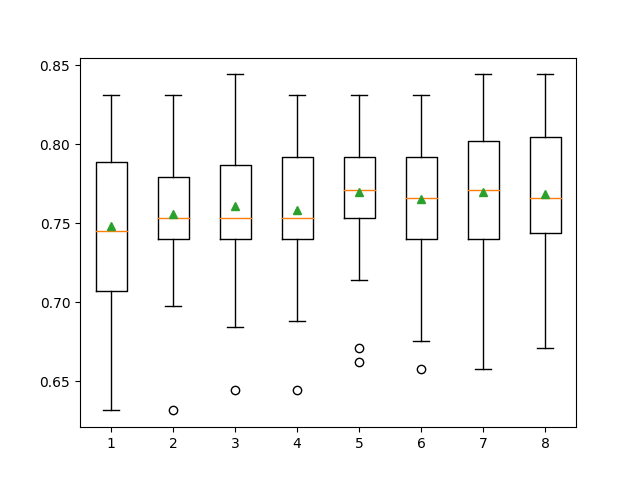
Nếu nhìn vào kết quả này thì k=5 sẽ tốt hơn k=7 vì mức độ phân tán (độ lệch chuẩn) của các gía trị độ chính xác trong các lần test khi k=5 nhỏ hơn khi k=7.

4. Kết luận

Bài thứ 3 về chủ đề Feature Selection, mình đã giới thiệu 2 kỹ thuật ANOVA F-Test và Mutual Information áp dụng cho Input Variables dạng Numerical. Toàn bộ code của bài này, các bạn có thể tham khảo tại đây.

Bài tiếp theo sẽ là các kỹ thuật Feature Selection áp dụng cho Output Variables dạng Numerical. Mời các bạn đón đọc.

5. Tham khảo

[1] Jason Brownlee, “Data Preparation for Machine Learning”, Book: https://machinelearningmastery.com/data-preparation-for-machine-learning/.

DP4ML - Feature Selection - Phần 3 - Select Numerical Input Features

1. Pima Indians Dataset

2. Numerical Feature Selection

2.1 ANOVA F-Test (Statistic)

2.2 Mutual Information Feature Selection

3. Modeling With Selected Features

3.1 Base model

3.2 Model Built Using ANOVA F-test Features

3.3 Model Built Using Mutual Information Features

3.4 Tune the Number of Selected Features

4. Kết luận

5. Tham khảo