SuNT's Blog | AI in Practical

Bài thứ 7 trong chuỗi các bài viết về chủ đề Data Preparation cho các mô hình ML và là bài thứ 4 về chủ đề Missing Data. Trong bài này, chúng ta sẽ tìm hiểu phương pháp tiếp theo để giải quyết vấn đề Missing Data, đó là phương pháp Iterative Imputation.

1. Iterative Imputation

Iterative Imputation là quá trình trong đó mỗi feature được mô hình hóa như một hàm của các features khác. Mỗi feature được xác định một cách tuần tự, lần lượt, cho phép các features đã xác định trước đó được sử dụng như làm một phần đầu vào của mô hình trong việc dự đoán các features tiếp theo. Quá trình này được lặp lại nhiều lần, cho phép các ước tính luôn được cải thiện. Cách tiếp cận này được gọi chung là Fully Conditional Specification (FCS) hoặc Multivariate Imputation by Chained Equations (MICE).

Về mặt lý thuyết, các thuật toán Regressions đều có thể sử dụng để ước lượng các Missing Data. Nhưng thực tế thì Linear Regression được sử dụng phổ biến vì tính đơn giản của nó. Số lượng vòng lặp cũng không cần quá lớn, thường là 10. Cuối cùng, thứ tự các features được ước lượng tuần tự cũng cần được xem xét. Có thể là từ các features có ít đến các features có nhiều Missing Data, hoặc là ngược lại.

2. Thực hành Iterative Imputation

Chúng ta sẽ thực hành phương pháp Iterative Imputation trên bộ dữ liệu Horse Colic Dataset giống như bài trước.

Thư viện Scikit-learn cung cấp lớp IterativeImputer giúp chúng ta dễ dàng thực hiện Iterative Imputation.

2.1 IterativeImputer và Data Transform

Cũng giống như SimpleImputer và kNNImputer, khi sử dụng IterativeImputer, nó sẽ tạo ra một phiên bản khác của tập dữ liệu ban đầu mà ở đó, các Missing Data đã được thay thế bởi các giá trị sinh ra từ thuật toán ước lượng (Data Transform). Các bước thực hiện Data Transform sử dụng IterativeImputer như sau:

a, Khai báo một Instance của IterativeImputer

Khi khởi tạo Instance cho IterativeImputer cần quan tâm đến 3 tham số truyền vào:

Thuật toán ước lượng (estimator): mặc định là ‘BayesianRidge’.
Thứ tự thực hiện ước lượng (imputation_order): mặc định là ‘ascending’, tức là từ các features có ít đến các features có nhiều Missing Data. Ngoài ra còn có các giá trị khác như: descending - từ các features có nhiều đến các features có ít Missing Data, roman - từ trái sang phải, arabic - từ phải sang trái, random - ngẫu nhiên.
Số lượng vòng lặp (max_iter): mặc định là 10.

...
# define imputer
imputer = IterativeImputer(estimator=BayesianRidge(), imputation_order= 'ascending')

b, Ước lượng giá trị cho Missing Data trên tập dữ liệu

...
# fit on the dataset
imputer.fit(X)

c, Tạo ra Transform Data

...
# transform the dataset
Xtrans = imputer.transform(X)

Để kiểm chứng lại hiệu quả làm việc của IterativeImputer, chúng ta sẽ áp dụng lên tập dữ liệu Horse Colic Dataset, xem trước và sau khi áp dụng IterativeImputer có gì thay đổi:

# iterative imputation transform for the horse colic dataset
from numpy import isnan
from pandas import read_csv
from sklearn.experimental import enable_iterative_imputer
from sklearn.impute import IterativeImputer
# load dataset
dataframe = read_csv('horse-colic.csv', header=None, na_values='?')
# split into input and output elements
data = dataframe.values
ix = [i for i in range(data.shape[1]) if i != 23]
X, y = data[:, ix], data[:, 23]
# summarize total missing
print('Missing: %d' % sum(isnan(X).flatten()))
# define imputer
imputer = IterativeImputer()
# fit on the dataset
imputer.fit(X)
# transform the dataset
Xtrans = imputer.transform(X)
# summarize total missing
print('Missing: %d' % sum(isnan(Xtrans).flatten()))

Kết quả:

Missing: 1605
Missing: 0

Ban đầu có 1605 Missing Data. Sau khi áp dụng IterativeImputer, số lượng Missing Data giảm về 0, chứng tỏ rằng nó đã thành công trong việc xóa bỏ Missing Data.

2.2 IterativeImputer và Model Evaluation

Phần này chúng ta sẽ áp dụng Iterative Imputation vào việc mô hình hóa thuật toán RandomForest trên tập dữ liệu Horse Colic Dataset. k-Fold Cross-validation và Pipleline cũng sẽ được sử dụng tương tự như bài trước.

# evaluate iterative imputation and random forest for the horse colic dataset
from numpy import mean
from numpy import std
from pandas import read_csv
from sklearn.ensemble import RandomForestClassifier
from sklearn.experimental import enable_iterative_imputer
from sklearn.impute import IterativeImputer
from sklearn.model_selection import cross_val_score
from sklearn.model_selection import RepeatedStratifiedKFold
from sklearn.pipeline import Pipeline
# load dataset
dataframe = read_csv('horse-colic.csv', header=None, na_values='?')
# split into input and output elements
data = dataframe.values
ix = [i for i in range(data.shape[1]) if i != 23]
X, y = data[:, ix], data[:, 23]
# define modeling pipeline
model = RandomForestClassifier()
imputer = IterativeImputer()
pipeline = Pipeline(steps=[('i', imputer), ('m', model)])
# define model evaluation
cv = RepeatedStratifiedKFold(n_splits=10, n_repeats=3, random_state=1)
# evaluate model
scores = cross_val_score(pipeline, X, y, scoring='accuracy', cv=cv, n_jobs=-1)
print('Mean Accuracy: %.3f (%.3f)' % (mean(scores), std(scores)))

Kết quả thực hiện:

Mean Accuracy: 0.871 (0.052)

2.3 Tuning imputation_order parameter

Như đã trình bày ở phần trên, imputation_order là một tham số quan trọng ảnh hưởng đến độ chính xác của IterativeImputer. Chúng ta không thể biết chính xác giá trị phù hợp nhất của nó đối với mỗi bộ dữ liệu. Cách dễ nhất để tìm ra nó là thử-sai, tức là chọn các giá trị có thể có của nó và thử lần lượt từng giá trị đó xem giá trị nào tốt nhất. Code dưới đây đánh giá độ chính xác trung bình của RandomForest cho mỗi trường hợp giá trị của imputation_order.

# compare iterative imputation strategies for the horse colic dataset
from numpy import mean
from numpy import std
from pandas import read_csv
from sklearn.ensemble import RandomForestClassifier
from sklearn.experimental import enable_iterative_imputer
from sklearn.impute import IterativeImputer
from sklearn.model_selection import cross_val_score
from sklearn.model_selection import RepeatedStratifiedKFold
from sklearn.pipeline import Pipeline
from matplotlib import pyplot
# load dataset
dataframe = read_csv('horse-colic.csv', header=None, na_values='?')
# split into input and output elements
data = dataframe.values
ix = [i for i in range(data.shape[1]) if i != 23]
X, y = data[:, ix], data[:, 23]
# evaluate each strategy on the dataset
results = list()
strategies = ['ascending', 'descending', 'roman', 'arabic', 'random']
for s in strategies:
	# create the modeling pipeline
	pipeline = Pipeline(steps=[('i', IterativeImputer(imputation_order=s)), ('m', RandomForestClassifier())])
	# evaluate the model
	cv = RepeatedStratifiedKFold(n_splits=10, n_repeats=3, random_state=1)
	scores = cross_val_score(pipeline, X, y, scoring='accuracy', cv=cv, n_jobs=-1)
	# store results
	results.append(scores)
	print('>%s %.3f (%.3f)' % (s, mean(scores), std(scores)))
# plot model performance for comparison
pyplot.boxplot(results, labels=strategies, showmeans=True)
pyplot.show()

Kết quả chạy:

Độ chính xác trung bình và độ lệch chuẩn.

>ascending 0.871 (0.054)
>descending 0.868 (0.051)
>roman 0.866 (0.054)
>arabic 0.864 (0.052)
>random 0.867 (0.049)

Theo kết quả này, độ chính xác khi imputation_order = ‘ascending’ cao nhất, nhưng độ lệch chuẩn cũng khá cao. imputation_order = ‘arabic cho ra độ chính xác thấp nhất, độ lệch chuẩn cao gần nhất.

Phân phối kết quả

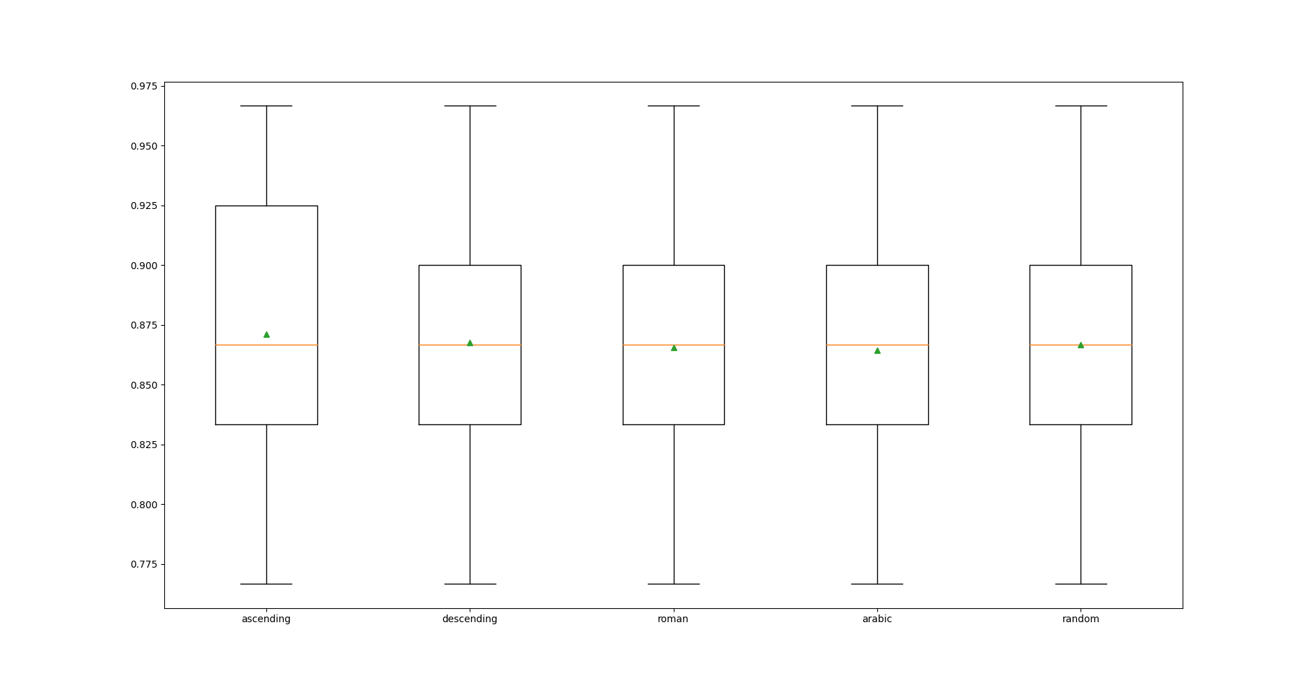
Mức độ phân phối trong trường hợp imputation_order = ‘ascending’ là lớn nhất.

Kết hợp các nhận xét trên, có thể nhận định imputation_order = ‘ascending’ là giá trị tối ưu của bài toán này.

2.4 Tuning max_iter parameter

Ngoài imputation_order thì max_iter cũng là 1 tham số ảnh hưởng đến độ chính xác của IterativeImputer. Code dưới đây đánh giá độ chính xác trung bình của RandomForest cho mỗi trường hợp giá trị của max_iter, từ 1 đến 20.

# compare iterative imputation number of iterations for the horse colic dataset
from numpy import mean
from numpy import std
from pandas import read_csv
from sklearn.ensemble import RandomForestClassifier
from sklearn.experimental import enable_iterative_imputer
from sklearn.impute import IterativeImputer
from sklearn.model_selection import cross_val_score
from sklearn.model_selection import RepeatedStratifiedKFold
from sklearn.pipeline import Pipeline
from matplotlib import pyplot
# load dataset
dataframe = read_csv('horse-colic.csv', header=None, na_values='?')
# split into input and output elements
data = dataframe.values
ix = [i for i in range(data.shape[1]) if i != 23]
X, y = data[:, ix], data[:, 23]
# evaluate each strategy on the dataset
results = list()
strategies = [str(i) for i in range(1, 21)]
for s in strategies:
	# create the modeling pipeline
	pipeline = Pipeline(steps=[('i', IterativeImputer(max_iter=int(s))), ('m', RandomForestClassifier())])
	# evaluate the model
	cv = RepeatedStratifiedKFold(n_splits=10, n_repeats=3, random_state=1)
	scores = cross_val_score(pipeline, X, y, scoring='accuracy', cv=cv, n_jobs=-1)
	# store results
	results.append(scores)
	print('>%s %.3f (%.3f)' % (s, mean(scores), std(scores)))
# plot model performance for comparison
pyplot.boxplot(results, labels=strategies, showmeans=True)
pyplot.show()

Kết quả chạy:

Độ chính xác trung bình và độ lệch chuẩn.

>1 0.869 (0.052)
>2 0.873 (0.053)
>3 0.869 (0.052)
>4 0.876 (0.053)
>5 0.874 (0.051)
>6 0.873 (0.051)
>7 0.870 (0.050)
>8 0.870 (0.050)
>9 0.866 (0.047)
>10 0.874 (0.059)
>11 0.870 (0.050)
>12 0.867 (0.049)
>13 0.873 (0.053)
>14 0.873 (0.055)
>15 0.871 (0.056)
>16 0.869 (0.050)
>17 0.874 (0.052)
>18 0.869 (0.056)
>19 0.876 (0.053)
>20 0.874 (0.055)

Theo kết quả này, độ chính xác khi max_iter = 4 hoặc 19 cao nhất.

Phân phối kết quả

Mức độ phân phối trong trường hợp max_iter = 4’ nhỏ hơn so với max_iter = 4.

Kết hợp các nhận xét trên, có thể nhận định max_iter = 19' là giá trị tối ưu của bài toán này.

2.5 Sử dụng IterativeImputer Transform khi dự đoán dữ liệu mới.

Chúng ta sẽ sử dụng các kết quả phân tích từ phần trên để tạo ra model, sau đó dự dự đoán trên một mẫu dữ liệu mới. Code hoàn chỉnh như sau:

# compare iterative imputation number of iterations for the horse colic dataset
# iterative imputation strategy and prediction for the horse colic dataset
from numpy import nan
from pandas import read_csv
from sklearn.ensemble import RandomForestClassifier
from sklearn.experimental import enable_iterative_imputer
from sklearn.impute import IterativeImputer
from sklearn.pipeline import Pipeline
# load dataset
dataframe = read_csv('horse-colic.csv', header=None, na_values='?')
# split into input and output elements
data = dataframe.values
ix = [i for i in range(data.shape[1]) if i != 23]
X, y = data[:, ix], data[:, 23]
# create the modeling pipeline
pipeline = Pipeline(steps=[('i', IterativeImputer(max_iter=19, imputation_order='ascending')), ('m', RandomForestClassifier())])
# fit the model
pipeline.fit(X, y)
# define new data
row = [2, 1, 530101, 38.50, 66, 28, 3, 3, nan, 2, 5, 4, 4, nan, nan, nan, 3, 5, 45.00, 8.40, nan, nan, 2, 11300, 00000, 00000, 2]
# make a prediction
yhat = pipeline.predict([row])
# summarize prediction
print('Predicted Class: %d' % yhat[0])

Kết quả thực hiện:

Predicted Class: 2

Chú ý quan trọng là Missing Data trong mẫu dữ liệu mới phải được đánh dấu là nan thì model mới có thể hiểu được.

3. Kết luận

Hôm nay, chúng ta đã tìm hiểu về phương pháp Iterative Imputation trong việc giải quyết vấn đề Missing Data. Đây là một phương pháp phức tạp hơn 3 phương pháp trước đó, nhưng thường mang lại hiệu quả cao hơn.

Toàn bộ code của bài này, các bạn có thể tham khảo tại đây.

Trong bài tiếp theo, chúng ta sẽ chuyển sang tìm hiểu một vấn đề mới của quá trình Data Prepration, đó là Feature Selection. Mời các bạn đón đọc.

4. Tham khảo

[1] Jason Brownlee, “Data Preparation for Machine Learning”, Book: https://machinelearningmastery.com/data-preparation-for-machine-learning/.

DP4ML - Missing Data - Phần 4 - Iterative Imputation