SuNT's Blog | AI in Practical

Ở bài trước, chúng ta đã áp dụng Autoencoders model vào bài toán Data Denoising. Trong bài này, chúng ta sẽ tiếp tục cùng nhau tìm hiểu 1 ứng dụng nữa của Autoencoders model trong bài toán Abnormal/Outline Data Detection.

1. Thế nào là Abnormal/Outline Data?

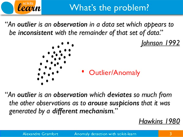
Đầu tiên, chúng ta cần hiểu rõ thế nào là Abnormal/Outline Data? Hiểu một cách đơn giản thì Abnormal/Outline Data là những dữ liệu mà khác với đa số phần dữ liệu còn lại. Cái “khác” có thể được thể hiện một cách trực quan qua đồ thị phân phối dạng Histogram, Scatter, …

Mặc dù thông thường tỷ lệ Abnormal/Outline Data rất nhỏ (cỡ < 1%) nhưng lại có tác hại rất lớn đến chất lương của model. Vì thế, nếu có thể phát hiện và loại bỏ được chúng thì có thể tạo ra được những model tốt.

Trong bài toán triển khai AI model vào thực tế, Abnormal/Outline Data còn được gọi là hiện tượng Data Driff. Đó là hiện tượng khi mà model đã hoạt động được một thời gian, đến một thời điểm nào đó, độ chính xác của model giảm xuống mà nguyên nhân là do dữ liệu mới đưa vào model không giống như dữ liệu lúc đầu huấn luyện tạo ra model. Nếu chúng ta phát hiện được sớm hiện tượng này và cập nhật lại model theo dữ liệu mới (chính là Abnormal/Outline Data) thì sẽ tiếp tục duy trì được sự ổn định của model.

Hiện tại, có khá nhiều thuật toán có thể sử dụng để phát hiện ra Abnormal/Outline Data, ví dụ như Isolation Forests, One-class SVMs, Elliptic Envelopes, Local Outlier Factor, hay thậm chí là sử dụng một DL model(CNN).

2. Sử dụng Autoencoders model cho bài toán Abnormal/Outline Data Detection

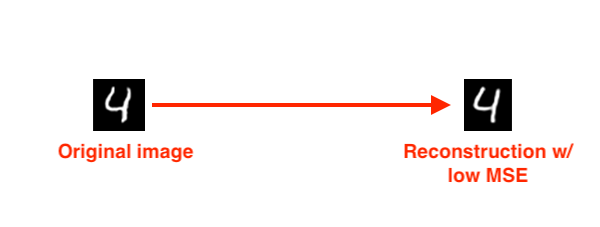
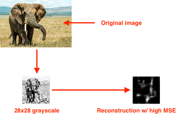
Để sử dụng Autoencoders model cho bài toàn Abnormal/Outline Data Detection, chúng ta căn cứ vào MSE giữa Output của Decoder và Input Data. Giả sử chúng ta đã huấn luyện được một Autoencoders model khá tốt, đạt được MSE nhỏ trên tập dữ liệu huấn luyện cũng như tập dữ liệu test. Bây giờ, nếu chúng ta đưa vào Encoder một dữ liệu mà khi tính MSE giữa dữ liệu đầu vào đó với Output của Decoder cho ra một giá trị tương đối lớn thì chúng ta có thể kết luận rằng, dữ liệu đầu vào đó là Abnormal/Outline Data.

Bây giờ chúng ta sẽ viết code để thực hiện việc này.

Cấu trúc thư mục làm việc như sau:

$ tree --dirsfirst
.
├── output
│   ├── autoencoder.model
│   └── images.pickle
├── sunt
│   ├── __init__.py
│   └── conv_autoencoder.py
├── find_anomalies.py
├── plot.png
├── recon_vis.png
└── train_unsupervised_autoencoder.py

File conv_autoencoder.py vẫn chứa định nghĩa Autoencoders model như những bài trước.

File train_unsupervised_autoencoder.py chứa code để huấn luyện model trên tập MNIST. Cụ thể là ở bài toán này, chúng ta chỉ sử dụng những ảnh chứa ký tự 1, còn những ảnh chứa ký tự khác sẽ được coi như là Abnormal/Outline Data. Kết quả huấn luyện sẽ là:

autoencoder.model: Autoencoders model đã huấn luyện.
images.pickle: Tập các images không có nhãn để tìm Abnormal/Outline Images trong đó.
plot.png: Đồ thị Loss trong quá trình huấn luyện.
recon_vis.png: So sánh Output của model với ảnh gốc ban đầu.

File find_anomalies.py chứa code để tìm ra Abnormal/Outline Images trong images.pickle.

Code của file train_unsupervised_autoencoder.py như sau:

# USAGE
# python train_unsupervised_autoencoder.py --dataset output/images.pickle --model output/autoencoder.model

# set the matplotlib backend so figures can be saved in the background
import matplotlib
matplotlib.use("Agg")

from tensorflow.compat.v1 import ConfigProto
from tensorflow.compat.v1 import InteractiveSession

config = ConfigProto()
config.gpu_options.allow_growth = True
session = InteractiveSession(config=config)

# import the necessary packages
from sunt.conv_autoencoder import ConvAutoencoder
from tensorflow.keras.optimizers import Adam
from tensorflow.keras.datasets import mnist
from sklearn.model_selection import train_test_split
import matplotlib.pyplot as plt
import numpy as np
import argparse
import random
import pickle
import cv2

def build_unsupervised_dataset(data, labels, validLabel=1,
	anomalyLabel=3, contam=0.01, seed=42):
	# grab all indexes of the supplied class label that are *truly* that particular label, then grab the indexes of the image labels that will serve as our "anomalies"
	validIdxs = np.where(labels == validLabel)[0]
	anomalyIdxs = np.where(labels == anomalyLabel)[0]

	# randomly shuffle both sets of indexes
	random.shuffle(validIdxs)
	random.shuffle(anomalyIdxs)

	# compute the total number of anomaly data points to select	i = int(len(validIdxs) * contam)
	anomalyIdxs = anomalyIdxs[:i]

	# use NumPy array indexing to extract both the valid images and "anomlay" images
	validImages = data[validIdxs]
	anomalyImages = data[anomalyIdxs]

	# stack the valid images and anomaly images together to form a single data matrix and then shuffle the rows
	images = np.vstack([validImages, anomalyImages])
	np.random.seed(seed)
	np.random.shuffle(images)

	# return the set of images
	return images

def visualize_predictions(decoded, gt, samples=10):
	# initialize our list of output images
	outputs = None

	# loop over our number of output samples
	for i in range(0, samples):
		# grab the original image and reconstructed image
		original = (gt[i] * 255).astype("uint8")
		recon = (decoded[i] * 255).astype("uint8")

		# stack the original and reconstructed image side-by-side
		output = np.hstack([original, recon])

		# if the outputs array is empty, initialize it as the current side-by-side image display
		if outputs is None:
			outputs = output

		# otherwise, vertically stack the outputs
		else:
			outputs = np.vstack([outputs, output])

	# return the output images
	return outputs

# construct the argument parse and parse the arguments
ap = argparse.ArgumentParser()
ap.add_argument("-d", "--dataset", type=str, required=True,
	help="path to output dataset file")
ap.add_argument("-m", "--model", type=str, required=True,
	help="path to output trained autoencoder")
ap.add_argument("-v", "--vis", type=str, default="recon_vis.png",
	help="path to output reconstruction visualization file")
ap.add_argument("-p", "--plot", type=str, default="plot.png",
	help="path to output plot file")
args = vars(ap.parse_args())

# initialize the number of epochs to train for, initial learning rate, and batch size
EPOCHS = 20
INIT_LR = 1e-3
BS = 32

# load the MNIST dataset
print("[INFO] loading MNIST dataset...")
((trainX, trainY), (testX, testY)) = mnist.load_data()

# build our unsupervised dataset of images with a small amount of contamination (i.e., anomalies) added into it
print("[INFO] creating unsupervised dataset...")
images = build_unsupervised_dataset(trainX, trainY, validLabel=1,
	anomalyLabel=3, contam=0.01)

# add a channel dimension to every image in the dataset, then scale the pixel intensities to the range [0, 1]
images = np.expand_dims(images, axis=-1)
images = images.astype("float32") / 255.0

# construct the training and testing split
(trainX, testX) = train_test_split(images, test_size=0.2,
	random_state=42)

# construct our convolutional autoencoder
print("[INFO] building autoencoder...")
(encoder, decoder, autoencoder) = ConvAutoencoder.build(28, 28, 1)
opt = Adam(lr=INIT_LR, decay=INIT_LR / EPOCHS)
autoencoder.compile(loss="mse", optimizer=opt)

# train the convolutional autoencoder
H = autoencoder.fit(
	trainX, trainX,
	validation_data=(testX, testX),
	epochs=EPOCHS,
	batch_size=BS)

# use the convolutional autoencoder to make predictions on the testing images, construct the visualization, and then save it to disk
print("[INFO] making predictions...")
decoded = autoencoder.predict(testX)
vis = visualize_predictions(decoded, testX)
cv2.imwrite(args["vis"], vis)

# construct a plot that plots and saves the training history
N = np.arange(0, EPOCHS)
plt.style.use("ggplot")
plt.figure()
plt.plot(N, H.history["loss"], label="train_loss")
plt.plot(N, H.history["val_loss"], label="val_loss")
plt.title("Training Loss")
plt.xlabel("Epoch #")
plt.ylabel("Loss")
plt.legend(loc="lower left")
plt.savefig(args["plot"])

# serialize the image data to disk
print("[INFO] saving image data...")
f = open(args["dataset"], "wb")
f.write(pickle.dumps(images))
f.close()

# serialize the autoencoder model to disk
print("[INFO] saving autoencoder...")
autoencoder.save(args["model"], save_format="h5")

Để cho giống với bài toán thực tế, mình chọn 99% hình ảnh chứa ký tự 1 và 1% hình ảnh chứa ký tự 3. Ký tự 3 coi như là Abnormal/Outline Data.

Trên Terminal, thực hiện lệnh sau:

$ python train_unsupervised_autoencoder.py --dataset output/images.pickle --model output/autoencoder.model
[INFO] loading MNIST dataset...
[INFO] creating unsupervised dataset...
[INFO] building autoencoder...
Epoch 1/20
2021-03-11 00:42:17.826156: I tensorflow/stream_executor/platform/default/dso_loader.cc:48] Successfully opened dynamic library libcublas.so.10
2021-03-11 00:42:17.981520: I tensorflow/stream_executor/platform/default/dso_loader.cc:48] Successfully opened dynamic library libcudnn.so.7
171/171 [==============================] - 1s 7ms/step - loss: 0.0428 - val_loss: 0.0468
Epoch 2/20
171/171 [==============================] - 1s 6ms/step - loss: 0.0076 - val_loss: 0.0347
Epoch 3/20
171/171 [==============================] - 1s 5ms/step - loss: 0.0039 - val_loss: 0.0129
Epoch 4/20
171/171 [==============================] - 1s 5ms/step - loss: 0.0033 - val_loss: 0.0035
Epoch 5/20
171/171 [==============================] - 1s 5ms/step - loss: 0.0029 - val_loss: 0.0029
Epoch 6/20
171/171 [==============================] - 1s 5ms/step - loss: 0.0027 - val_loss: 0.0028
Epoch 7/20
171/171 [==============================] - 1s 5ms/step - loss: 0.0024 - val_loss: 0.0028
Epoch 8/20
171/171 [==============================] - 1s 5ms/step - loss: 0.0023 - val_loss: 0.0028
Epoch 9/20
171/171 [==============================] - 1s 6ms/step - loss: 0.0022 - val_loss: 0.0025
Epoch 10/20
171/171 [==============================] - 1s 4ms/step - loss: 0.0021 - val_loss: 0.0024
Epoch 11/20
171/171 [==============================] - 1s 5ms/step - loss: 0.0020 - val_loss: 0.0024
Epoch 12/20
171/171 [==============================] - 1s 6ms/step - loss: 0.0020 - val_loss: 0.0023
Epoch 13/20
171/171 [==============================] - 1s 4ms/step - loss: 0.0019 - val_loss: 0.0024
Epoch 14/20
171/171 [==============================] - 1s 5ms/step - loss: 0.0018 - val_loss: 0.0022
Epoch 15/20
171/171 [==============================] - 1s 4ms/step - loss: 0.0019 - val_loss: 0.0023
Epoch 16/20
171/171 [==============================] - 1s 6ms/step - loss: 0.0018 - val_loss: 0.0022
Epoch 17/20
171/171 [==============================] - 1s 5ms/step - loss: 0.0017 - val_loss: 0.0022
Epoch 18/20
171/171 [==============================] - 1s 5ms/step - loss: 0.0017 - val_loss: 0.0022
Epoch 19/20
171/171 [==============================] - 1s 6ms/step - loss: 0.0017 - val_loss: 0.0021
Epoch 20/20
171/171 [==============================] - 1s 6ms/step - loss: 0.0016 - val_loss: 0.0022
[INFO] making predictions...
[INFO] saving image data...
[INFO] saving autoencoder...

Đồ thị Loss trong quá trình huấn luyện:

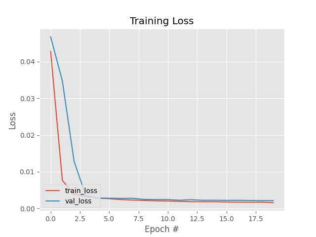
Loss trên 2 tập Training và Validation khá tương đồng, hầu như không có hiện tượng Overfitting.

So sánh Input Data và Output của model:

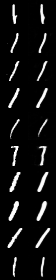
Sau khi có được Autoencoders model đã huấn luyện, ta thử đi tìm Abnormal/Outline Images. Code cho file find_anomalies.py như sau:

# USAGE
# python find_anomalies.py --dataset output/images.pickle --model output/autoencoder.model

# import the necessary packages
from tensorflow.keras.models import load_model
import numpy as np
import argparse
import pickle
import cv2

from tensorflow.compat.v1 import ConfigProto
from tensorflow.compat.v1 import InteractiveSession

config = ConfigProto()
config.gpu_options.allow_growth = True
session = InteractiveSession(config=config)

# construct the argument parse and parse the arguments
ap = argparse.ArgumentParser()
ap.add_argument("-d", "--dataset", type=str, required=True,
	help="path to input image dataset file")
ap.add_argument("-m", "--model", type=str, required=True,
	help="path to trained autoencoder")
ap.add_argument("-q", "--quantile", type=float, default=0.999,
	help="q-th quantile used to identify outliers")
args = vars(ap.parse_args())

# load the model and image data from disk
print("[INFO] loading autoencoder and image data...")
autoencoder = load_model(args["model"])
images = pickle.loads(open(args["dataset"], "rb").read())

# make predictions on our image data and initialize our list of reconstruction errors
decoded = autoencoder.predict(images)
errors = []

# loop over all original images and their corresponding reconstructions
for (image, recon) in zip(images, decoded):
	# compute the mean squared error between the ground-truth image and the reconstructed image, then add it to our list of errors
	mse = np.mean((image - recon) ** 2)
	errors.append(mse)

# compute the q-th quantile of the errors which serves as our threshold to identify anomalies -- any data point that our model reconstructed with > threshold error will be marked as an outlier
thresh = np.quantile(errors, args["quantile"])
idxs = np.where(np.array(errors) >= thresh)[0]
print("[INFO] mse threshold: {}".format(thresh))
print("[INFO] {} outliers found".format(len(idxs)))

# initialize the outputs array
outputs = None

# loop over the indexes of images with a high mean squared error term
for i in idxs:
	# grab the original image and reconstructed image
	original = (images[i] * 255).astype("uint8")
	recon = (decoded[i] * 255).astype("uint8")

	# stack the original and reconstructed image side-by-side
	output = np.hstack([original, recon])

	# if the outputs array is empty, initialize it as the current side-by-side image display
	if outputs is None:
		outputs = output

	# otherwise, vertically stack the outputs
	else:
		outputs = np.vstack([outputs, output])

# show the output visualization
cv2.imshow("Output", outputs)
cv2.waitKey(0)

Để tính toán ngưỡng MSE cho việc phân loại dữ liệu là Abnormal/Outline Data hay không, chúng ta sử dụng Quantile với p = 0.999.

Thực hiện lệnh sau trên Terminal để tìm Abnorlmal/Ouline Images:

$ python find_anomalies.py --dataset output/images.pickle --model output/autoencoder.model
[INFO] loading autoencoder and image data...
[INFO] mse threshold: 0.03480463531613351
[INFO] 7 outliers found

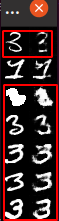
2 nhận xét:

Mặc dù Autoencoders model chỉ được huấn luyện với 1% dữ liệu chứa ký tự 3 (*trên tống số *) nhưng nó đã tái hiện lại khá tốt khi đưa hình ảnh chứa số 3 vào.
Những hình ảnh chứa ký tự 3 có giá trị MSE cao hơn ngưỡng và được xác định là Abnormal/Outline Data.

3. Kết luận

Trong bài này, chúng ta đã tìm hiểu về Abnormal/Outline Data và cách xây dựng một Autoencoders model để giải quyết nó.

Trong thực tế thì không có một phương pháp nào có thể phát hiện hoàn toàn Abnormal/Outline Data. Các bạn có thể tìm hiểu thêm một số phương pháp khác tại đây.

Toàn bộ Source Code của bài này, các bạn có thể xem tại github cá nhân của mình.

4. Tham khảo

Pyimagesearch