Sử dụng Autoencoders model cho bài toán Denoising Data
Ở bài trước, chúng ta đã tìm hiểu về Autoencoders model và một số ứng dụng của nó. Trong bài này, mình sẽ cũng các bạn sử dụng Autoencoders model để thực hiện việc giảm nhiễu cho dữ liệu hình ảnh. Việc này có thể áp dụng để tăng độ chính xác của hệ thống OCR bằng cách nâng cao chất lượng của ảnh đầu vào hệ thống.
1. Denoising Autoencoders
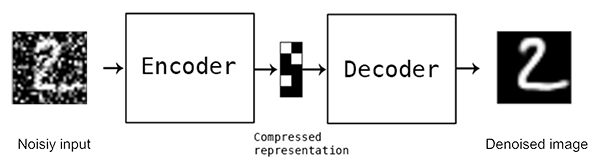
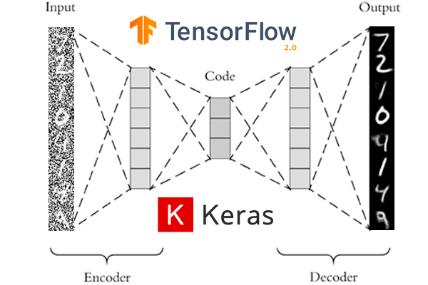
Về bản chất, Autoencoders model cho bài toán Denoising là sự mở rộng của Autoencoders model ở bài trước. Điểm khác biệt ở chỗ, Output của Decoder không phải là Input Data (có nhiễu) mà là Input Data (không có nhiễu).
Để chuẩn bị dữ liệu cho việc huấn luyện Autoencoders model phục vụ mục đích Denoising, ta có thể làm như sau:
- Chọn ra những dữ liệu (gọi là tập B) không có nhiễu từ tập dữ liệu đầy đủ ban đầu (tập A).
- Thêm nhiễu ngẫu nhiên vào tập B, tạo thành tập C.
- Huấn luyện Autoencoders model với Input Data là tập C, Output từ Decoder là tập B.
- Áp dụng Autoencoders model đã trên toàn bộ tập A.
2. Denoising Autoencoders với Keras và TensorFlow
Cấu trúc thư mục làm việc:
$ tree --dirsfirst
.
├── sunt
│   ├── __init__.py
│   └── conv_autoencoder.py
├── output.png
├── plot.png
└── train_denoising_autoencoder.py
Module sunt chứa lớp conv_autoencoder.py mà chúng ta đã sử dụng ở bài trước.
Trọng tâm của bài này nằm ở file train_denoising_autoencoder.py. Sử dụng tập dữ liệu MNIST, chúng ta thêm nhiễu vào rồi huấn luyện Autoencoders model. Ở đây, nhiễu được tạo ra bằng cách sinh ngẫu nhiên dữ liệu theo phân phối chuẩn có điểm trung tâm là 0.5, độ lệch chuẩn là 0.5. Toàn bộ code của file này như sau:
# USAGE
# python train_denoising_autoencoder.py

# set the matplotlib backend so figures can be saved in the background
import matplotlib
matplotlib.use("Agg")

from tensorflow.compat.v1 import ConfigProto
from tensorflow.compat.v1 import InteractiveSession

config = ConfigProto()
config.gpu_options.allow_growth = True
session = InteractiveSession(config=config)

# import the necessary packages
from sunt.conv_autoencoder import ConvAutoencoder
from tensorflow.keras.optimizers import Adam
from tensorflow.keras.datasets import mnist
import matplotlib.pyplot as plt
import numpy as np
import argparse
import cv2

# construct the argument parse and parse the arguments
ap = argparse.ArgumentParser()
ap.add_argument("-s", "--samples", type=int, default=8,
	help="# number of samples to visualize when decoding")
ap.add_argument("-o", "--output", type=str, default="output.png",
	help="path to output visualization file")
ap.add_argument("-p", "--plot", type=str, default="plot.png",
	help="path to output plot file")
args = vars(ap.parse_args())

# initialize the number of epochs to train for and batch size
EPOCHS = 25
BS = 32

# load the MNIST dataset
print("[INFO] loading MNIST dataset...")
((trainX, _), (testX, _)) = mnist.load_data()

# add a channel dimension to every image in the dataset, then scale the pixel intensities to the range [0, 1]
trainX = np.expand_dims(trainX, axis=-1)
testX = np.expand_dims(testX, axis=-1)
trainX = trainX.astype("float32") / 255.0
testX = testX.astype("float32") / 255.0

# sample noise from a random normal distribution centered at 0.5 (since our images lie in the range [0, 1]) and a standard deviation of 0.5
trainNoise = np.random.normal(loc=0.5, scale=0.5, size=trainX.shape)
testNoise = np.random.normal(loc=0.5, scale=0.5, size=testX.shape)
trainXNoisy = np.clip(trainX + trainNoise, 0, 1)
testXNoisy = np.clip(testX + testNoise, 0, 1)

# construct our convolutional autoencoder
print("[INFO] building autoencoder...")
(encoder, decoder, autoencoder) = ConvAutoencoder.build(28, 28, 1)
opt = Adam(lr=1e-3)
autoencoder.compile(loss="mse", optimizer=opt)

# train the convolutional autoencoder
H = autoencoder.fit(
	trainXNoisy, trainX,
	validation_data=(testXNoisy, testX),
	epochs=EPOCHS,
	batch_size=BS)

# construct a plot that plots and saves the training history
N = np.arange(0, EPOCHS)
plt.style.use("ggplot")
plt.figure()
plt.plot(N, H.history["loss"], label="train_loss")
plt.plot(N, H.history["val_loss"], label="val_loss")
plt.title("Training Loss and Accuracy")
plt.xlabel("Epoch #")
plt.ylabel("Loss/Accuracy")
plt.legend(loc="lower left")
plt.savefig(args["plot"])

# use the convolutional autoencoder to make predictions on the testing images, then initialize our list of output images
print("[INFO] making predictions...")
decoded = autoencoder.predict(testXNoisy)
outputs = None

# loop over our number of output samples
for i in range(0, args["samples"]):
	# grab the original image and reconstructed image
	original = (testXNoisy[i] * 255).astype("uint8")
	recon = (decoded[i] * 255).astype("uint8")

	# stack the original and reconstructed image side-by-side
	output = np.hstack([original, recon])

	# if the outputs array is empty, initialize it as the current side-by-side image display
	if outputs is None:
		outputs = output

	# otherwise, vertically stack the outputs
	else:
		outputs = np.vstack([outputs, output])

# save the outputs image to disk
cv2.imwrite(args["output"], outputs)
Thực hiện lệnh sau trên Terminer:
$ python train_denoising_autoencoder.py
2021-03-10 23:09:12.350152: I tensorflow/core/common_runtime/gpu/gpu_device.cc:1402] Created TensorFlow device (/job:localhost/replica:0/task:0/device:GPU:0 with 4932 MB memory) -> physical GPU (device: 0, name: GeForce GTX 1660 Ti with Max-Q Design, pci bus id: 0000:01:00.0, compute capability: 7.5)
[INFO] loading MNIST dataset...
[INFO] building autoencoder...
Epoch 1/25
2021-03-10 23:09:14.814333: I tensorflow/stream_executor/platform/default/dso_loader.cc:48] Successfully opened dynamic library libcublas.so.10
2021-03-10 23:09:14.963101: I tensorflow/stream_executor/platform/default/dso_loader.cc:48] Successfully opened dynamic library libcudnn.so.7
1875/1875 [==============================] - 7s 4ms/step - loss: 0.0276 - val_loss: 0.0195
Epoch 2/25
1875/1875 [==============================] - 7s 4ms/step - loss: 0.0187 - val_loss: 0.0213
Epoch 3/25
1875/1875 [==============================] - 7s 4ms/step - loss: 0.0177 - val_loss: 0.0182
Epoch 4/25
1875/1875 [==============================] - 8s 4ms/step - loss: 0.0172 - val_loss: 0.0181
Epoch 5/25
1875/1875 [==============================] - 7s 4ms/step - loss: 0.0167 - val_loss: 0.0185
Epoch 6/25
1875/1875 [==============================] - 7s 4ms/step - loss: 0.0164 - val_loss: 0.0167
Epoch 7/25
1875/1875 [==============================] - 7s 4ms/step - loss: 0.0162 - val_loss: 0.0161
Epoch 8/25
1875/1875 [==============================] - 7s 4ms/step - loss: 0.0160 - val_loss: 0.0162
Epoch 9/25
1875/1875 [==============================] - 7s 4ms/step - loss: 0.0158 - val_loss: 0.0159
Epoch 10/25
1875/1875 [==============================] - 7s 4ms/step - loss: 0.0156 - val_loss: 0.0166
Epoch 11/25
1875/1875 [==============================] - 7s 4ms/step - loss: 0.0155 - val_loss: 0.0164
Epoch 12/25
1875/1875 [==============================] - 7s 4ms/step - loss: 0.0154 - val_loss: 0.0157
Epoch 13/25
1875/1875 [==============================] - 7s 4ms/step - loss: 0.0153 - val_loss: 0.0158
Epoch 14/25
1875/1875 [==============================] - 7s 4ms/step - loss: 0.0152 - val_loss: 0.0167
Epoch 15/25
1875/1875 [==============================] - 7s 4ms/step - loss: 0.0151 - val_loss: 0.0157
Epoch 16/25
1875/1875 [==============================] - 7s 4ms/step - loss: 0.0150 - val_loss: 0.0155
Epoch 17/25
1875/1875 [==============================] - 7s 4ms/step - loss: 0.0149 - val_loss: 0.0160
Epoch 18/25
1875/1875 [==============================] - 7s 4ms/step - loss: 0.0149 - val_loss: 0.0174
Epoch 19/25
1875/1875 [==============================] - 7s 4ms/step - loss: 0.0148 - val_loss: 0.0155
Epoch 20/25
1875/1875 [==============================] - 7s 4ms/step - loss: 0.0147 - val_loss: 0.0155
Epoch 21/25
1875/1875 [==============================] - 7s 4ms/step - loss: 0.0147 - val_loss: 0.0157
Epoch 22/25
1875/1875 [==============================] - 7s 4ms/step - loss: 0.0146 - val_loss: 0.0154
Epoch 23/25
1875/1875 [==============================] - 7s 4ms/step - loss: 0.0146 - val_loss: 0.0156
Epoch 24/25
1875/1875 [==============================] - 7s 4ms/step - loss: 0.0145 - val_loss: 0.0156
Epoch 25/25
1875/1875 [==============================] - 7s 4ms/step - loss: 0.0145 - val_loss: 0.0154
[INFO] making predictions...
Đồ thị thể hiện quá trình huấn luyện:
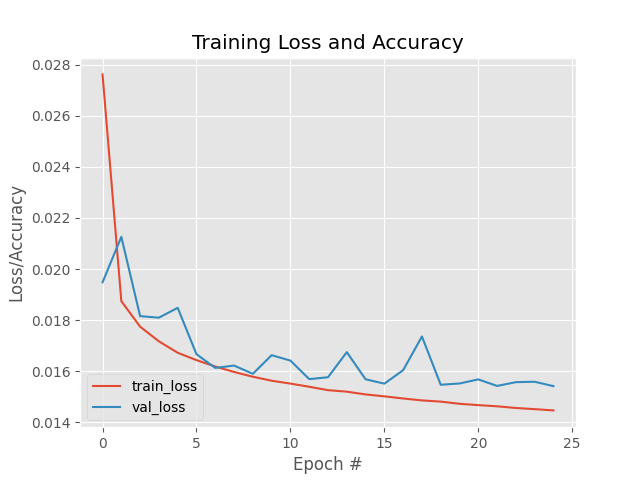
Ta thấy Train Loss và Validation Loss đều giảm dần khi số lượng epochs tăng và không xảy ra hiện tượng Overfitting.
Ảnh mới sinh ra từ Autoencoders model so với ảnh đưa vào:
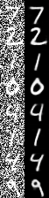
Bên trái là Input Data, còn bên phải là Output của Autoencoder model. Ta thấy rất rõ, nhiễu đã được khử gần như hoàn toàn.
3. Kết luận
Trong bài này, chúng ta đã cùng xây dựng một Autoencoders model để phục vụ mục đích giảm nhiễu của dữ liệu. Đây là một trong những ứng dụng rất hay của Autoencoders model, giúp nâng cao chất lượng dữ liệu trước khi đưa vào huấn luyện các mô hình DL khác, đặc biệt hữu ích trong bài toán OCR.
Toàn bộ Source Code của bài này, các bạn có thể tham khảo tại github cá nhân của mình tại đây.
Hẹn các bạn trong các bài viết tiếp theo.
4. Tham khảo