SuNT's Blog | AI in Practical

Loạt bài tiếp theo mình sẽ viết về kiến trúc Autoencoders và một số ứng dụng của chúng.

Bài đầu tiên, chúng ta sẽ thảo luận Autoencoders là gì, nó có gì khác so với các Generative models khác (ví dụ: GAN), những ứng dụng của chúng, … Mình cũng sẽ xây dựng một Autoencoders model đơn giản sử dụng Keras và Tensorflow.

1. Autoencoders là gì?

Autoencoders là một dạng của Unsupervised Neural Network. Hoạt động của nó được mô tả như sau:

Nhận một tập dữ liệu đầu vào (input data).
Chuyển đổi Input Data sang một dạng biểu diễn khác trong không gian tiềm ẩn (Latent Space).
Tái hiện lại Input Data từ Latent Space Representation.

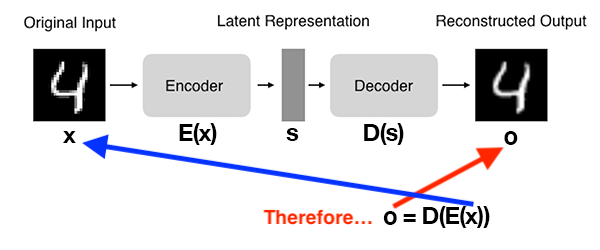
Xét về mặt cấu tạo, một Autoencoders model gồm 2 thành phần (subnetworks):

Encoder: Nhận Input Data rồi chuyển nó sang dạng khác trong Latent Space.

$s = E(x)$

Trong đó $x$ là Input Data, $E$ là Encoder, và $s$ là Output trong Latent Space.

Decoder: Nhận Output của Encoder trong Latent Space, $s$, và tái hiện lại Input Data.

$o = D(s)$

Trong đó, $o$ là Output của Decoder $D$.

Công thức chung cho toàn bộ quá trình Autoencoder sẽ là:

$o = D(E(x))$

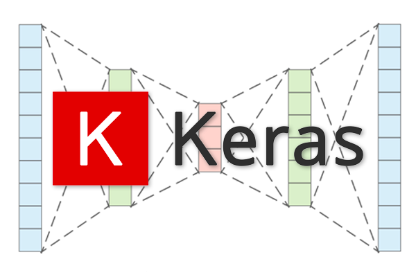
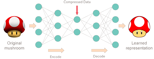
Kiến trúc tổng quát của Autoencoders được minh họa như sau:

Để huấn luyện Autoencoders model, chúng ta đưa cho nó Input Data, nó sẽ cố gắng tái hiện lại Input Data bằng cách tối thiểu hóa Mean Squared Error giữa Ouput của model và Input Data. Hay nói cách khác Input Data là nhãn của chính nó.

Một Autoencoders model lý tưởng khi Output của nó giống hệt với Input Data.

Liệu bạn có thắc mắc là tại sao chúng ta phải tạo ra Autoencoders model, đi một vòng chỉ để tái hiện lại Input Data? Sao ta không copy luôn Input Data ra là xong chuyện???

Mình cũng từng thắc mắc như bạn khi mới bắt đầu tìm hiểu về Autoencoders.

Nhưng bạn nên biết rằng, giá trị thực sự của Autoencoders model nằm ở Output của Encoder trong Latent Space. Hay nói cách khác, chúng ta (thường) chỉ quan tâm đến Encoder và Latent Space mà không quá quan tâm đến Decoder.

Một ví dụ để bạn dễ hình dung hơn. Giả sử chúng ta có một tập ảnh, mỗi ảnh có kích thước 28x28x1, tức là chúng ta phải sử dụng 28x28x1 = 784 bytes để lưu mỗi ảnh. Sử dụng Autoencoders model, chúng ta chuyển đổi ảnh đó sang một vector nhỏ hơn, chỉ còn 16 bytes trong Latent Space. Sử dụng 16 bytes của vector này, chúng ta sau đó có thể tái hiện lại ảnh ban đầu giống đến 98%. Điều này giúp ta tiết kiệm được rất nhiều không gian lưu trữ, đặc biệt khi phải truyền dữ liệu đó qua môi trường mạng Internet. Đó chính là một trong những ứng dụng của Autoencoders.

2. Ứng dụng của Autoencoders model

Kiến trúc tổng quát của Autoencoders được minh họa như sau:

Một số ứng dụng của Autoencoders trong lĩnh vực Computer Vision có thể kể đến như:

Giảm chiểu dữ liệu (Dimensionality Reduction): Ứng dụng này giống như thuật toán PCA nhưng hiệu quả hơn.
Giảm nhiễu dữ liệu (Denoising): Giảm nhiễu dữ liệu, một bước trong quá trình tiền xử lý ảnh, giúp nâng cao độ chính xác của hệ thống OCR.
Phát hiện bất thường (Anomaly/outlier Detection): Phát hiện những điểm dữ liệu bất thường trong tập dataset, ví dụ như thiết nhãn, lệch ra khỏi phân phối chung của toàn dữ liệu. Một khi đã phát hiện được dữ liệu bất thường, ta có thể loại bỏ chúng hoặc huấn luyện lại model để tăng độ chính xác.

Trong lĩnh vực Natual Language Processing (NLP), Autoencoders model giúp giải quyết các bài toán:

Tạo ra đoạn text miêu tả nội dung bức ảnh (Image Caption Generation)
Tóm tắt nội dung đoạn văn (Text Summarization)
Trích xuất đăc trưng (Word Embedding)

3. So sánh Autoencoders và Generative Adversarial Networks (GAN)

Nếu bạn biết về GAN, bạn có thể nhận thấy Autoencoders và GAN có sự tương đồng về cách làm việc. Cả 2 models đề thuộc dạng Generative.

Autoencoders: Nhận Input Data, chuyển thành một vector có số chiều nhỏ hơn trong Latent Space. Sau đó, cố gắng tái hiện lại Input Data từ các vector trong Latent Space.
GAN: Nhận Input Data có số chiều nhỏ, chuyển thành một vector có số chiều lớn hơn. Sau đó, sinh ra một dữ liệu mới từ vector này, đáp ứng một tiêu chí nào đó. Mình sẽ viết một series bài về GAN trong tương lai.

Chi tiết hơn về so sánh giữa Autoencoders và GAN, bạn có thể đọc tại đây.

4. Xây dựng một Autoencoders model đơn giản với Keras và Tensorflow

Chúng ta sẽ thử cùng nhau huấn luyện một Autoencoders model trên tập dữ liệu MNIST.

Cấu trúc thư mục làm việc như sau:

$ tree --dirsfirst
.
├── sunt
│   ├── __init__.py
│   └── conv_autoencoder.py
├── output.png
├── plot.png
└── train_conv_autoencoder.py

File conv_autoencoder.py: Chứa lớp ConvAutoencoder và phương thúc build để xây dựng kiến trúc mạng của Autoencoders model.
File train_conv_autoencoder.py: Huấn luyện Autoencoders model trên tập MINIST.

Mở file conv_autoencoder.py và viết code như sau:

# import the necessary packages
from tensorflow.keras.layers import BatchNormalization
from tensorflow.keras.layers import Conv2D
from tensorflow.keras.layers import Conv2DTranspose
from tensorflow.keras.layers import LeakyReLU
from tensorflow.keras.layers import Activation
from tensorflow.keras.layers import Flatten
from tensorflow.keras.layers import Dense
from tensorflow.keras.layers import Reshape
from tensorflow.keras.layers import Input
from tensorflow.keras.models import Model
from tensorflow.keras import backend as K
import numpy as np

class ConvAutoencoder:
	@staticmethod
	def build(width, height, depth, filters=(32, 64), latentDim=16):
		# initialize the input shape to be "channels last" along with the channels dimension itself channels dimension itself
		inputShape = (height, width, depth)
		chanDim = -1

		# define the input to the encoder
		inputs = Input(shape=inputShape)
		x = inputs

		# loop over the number of filters
		for f in filters:
			# apply a CONV => RELU => BN operation
			x = Conv2D(f, (3, 3), strides=2, padding="same")(x)
			x = LeakyReLU(alpha=0.2)(x)
			x = BatchNormalization(axis=chanDim)(x)

		# flatten the network and then construct our latent vector
		volumeSize = K.int_shape(x)
		x = Flatten()(x)
		latent = Dense(latentDim)(x)

		# build the encoder model
		encoder = Model(inputs, latent, name="encoder")
        print(encoder.summary())

		# start building the decoder model which will accept the output of the encoder as its inputs
		latentInputs = Input(shape=(latentDim,))
		x = Dense(np.prod(volumeSize[1:]))(latentInputs)
		x = Reshape((volumeSize[1], volumeSize[2], volumeSize[3]))(x)

		# loop over our number of filters again, but this time in reverse order
		for f in filters[::-1]:
			# apply a CONV_TRANSPOSE => RELU => BN operation
			x = Conv2DTranspose(f, (3, 3), strides=2,
				padding="same")(x)
			x = LeakyReLU(alpha=0.2)(x)
			x = BatchNormalization(axis=chanDim)(x)

		# apply a single CONV_TRANSPOSE layer used to recover the original depth of the image
		x = Conv2DTranspose(depth, (3, 3), padding="same")(x)
		outputs = Activation("sigmoid")(x)

		# build the decoder model
		decoder = Model(latentInputs, outputs, name="decoder")
        print(decoder.summary())

		# our autoencoder is the encoder + decoder
		autoencoder = Model(inputs, decoder(encoder(inputs)),
			name="autoencoder")
        print(autoencoder.summay())

		# return a 3-tuple of the encoder, decoder, and autoencoder
		return (encoder, decoder, autoencoder)

Mở file train_conv_autoencoder.py và viết code như sau:

# USAGE
# python train_conv_autoencoder.py

# set the matplotlib backend so figures can be saved in the background
import matplotlib
matplotlib.use("Agg")

from tensorflow.compat.v1 import ConfigProto
from tensorflow.compat.v1 import InteractiveSession

config = ConfigProto()
config.gpu_options.allow_growth = True
session = InteractiveSession(config=config)

# import the necessary packages
from sunt.convautoencoder import ConvAutoencoder
from tensorflow.keras.optimizers import Adam
from tensorflow.keras.datasets import mnist
import matplotlib.pyplot as plt
import numpy as np
import argparse
import cv2

# construct the argument parse and parse the arguments
ap = argparse.ArgumentParser()
ap.add_argument("-s", "--samples", type=int, default=8,
	help="# number of samples to visualize when decoding")
ap.add_argument("-o", "--output", type=str, default="output.png",
	help="path to output visualization file")
ap.add_argument("-p", "--plot", type=str, default="plot.png",
	help="path to output plot file")
args = vars(ap.parse_args())

# initialize the number of epochs to train for and batch size
EPOCHS = 25
BS = 32

# load the MNIST dataset
print("[INFO] loading MNIST dataset...")
((trainX, _), (testX, _)) = mnist.load_data()

# add a channel dimension to every image in the dataset, then scale
# the pixel intensities to the range [0, 1]
trainX = np.expand_dims(trainX, axis=-1)
testX = np.expand_dims(testX, axis=-1)
trainX = trainX.astype("float32") / 255.0
testX = testX.astype("float32") / 255.0

# construct our convolutional autoencoder
print("[INFO] building autoencoder...")
(encoder, decoder, autoencoder) = ConvAutoencoder.build(28, 28, 1)
opt = Adam(lr=1e-3)
autoencoder.compile(loss="mse", optimizer=opt)

# train the convolutional autoencoder
H = autoencoder.fit(
	trainX, trainX,
	validation_data=(testX, testX),
	epochs=EPOCHS,
	batch_size=BS)

# construct a plot that plots and saves the training history
N = np.arange(0, EPOCHS)
plt.style.use("ggplot")
plt.figure()
plt.plot(N, H.history["loss"], label="train_loss")
plt.plot(N, H.history["val_loss"], label="val_loss")
plt.title("Training Loss and Accuracy")
plt.xlabel("Epoch #")
plt.ylabel("Loss/Accuracy")
plt.legend(loc="lower left")
plt.savefig(args["plot"])

# use the convolutional autoencoder to make predictions on the
# testing images, then initialize our list of output images
print("[INFO] making predictions...")
decoded = autoencoder.predict(testX)
outputs = None

# loop over our number of output samples
for i in range(0, args["samples"]):
	# grab the original image and reconstructed image
	original = (testX[i] * 255).astype("uint8")
	recon = (decoded[i] * 255).astype("uint8")

	# stack the original and reconstructed image side-by-side
	output = np.hstack([original, recon])

	# if the outputs array is empty, initialize it as the current
	# side-by-side image display
	if outputs is None:
		outputs = output

	# otherwise, vertically stack the outputs
	else:
		outputs = np.vstack([outputs, output])

# save the outputs image to disk
cv2.imwrite(args["output"], outputs)

Trong code đã có đầy đủ comments, hi vọng các bạn có thể hiểu được.

Tiến hành chạy code (mình dùng python 3.8, tensorflow 2.3.0 trong môi trường ảo anaconda):

$ python train_conv_autoencoder.py

Output:

Kiến trúc của Encoder:

Model: "encoder"
_________________________________________________________________
Layer (type)                 Output Shape              Param #   
=================================================================
input_1 (InputLayer)         [(None, 28, 28, 1)]       0         
_________________________________________________________________
conv2d (Conv2D)              (None, 14, 14, 32)        320       
_________________________________________________________________
leaky_re_lu (LeakyReLU)      (None, 14, 14, 32)        0         
_________________________________________________________________
batch_normalization (BatchNo (None, 14, 14, 32)        128       
_________________________________________________________________
conv2d_1 (Conv2D)            (None, 7, 7, 64)          18496     
_________________________________________________________________
leaky_re_lu_1 (LeakyReLU)    (None, 7, 7, 64)          0         
_________________________________________________________________
batch_normalization_1 (Batch (None, 7, 7, 64)          256       
_________________________________________________________________
flatten (Flatten)            (None, 3136)              0         
_________________________________________________________________
dense (Dense)                (None, 16)                50192     
=================================================================
Total params: 69,392
Trainable params: 69,200
Non-trainable params: 192

Ta thấy từ kiến trúc trên, Input Data ban đầu là 28x28x1 = 784 bytes, sau khi chuyển sang Latent Space, dữ liệu chỉ còn là vector 16 bytes.

Kiến trúc của Decoder:

Model: "decoder"
_________________________________________________________________
Layer (type)                 Output Shape              Param #   
=================================================================
input_2 (InputLayer)         [(None, 16)]              0         
_________________________________________________________________
dense_1 (Dense)              (None, 3136)              53312     
_________________________________________________________________
reshape (Reshape)            (None, 7, 7, 64)          0         
_________________________________________________________________
conv2d_transpose (Conv2DTran (None, 14, 14, 64)        36928     
_________________________________________________________________
leaky_re_lu_2 (LeakyReLU)    (None, 14, 14, 64)        0         
_________________________________________________________________
batch_normalization_2 (Batch (None, 14, 14, 64)        256       
_________________________________________________________________
conv2d_transpose_1 (Conv2DTr (None, 28, 28, 32)        18464     
_________________________________________________________________
leaky_re_lu_3 (LeakyReLU)    (None, 28, 28, 32)        0         
_________________________________________________________________
batch_normalization_3 (Batch (None, 28, 28, 32)        128       
_________________________________________________________________
conv2d_transpose_2 (Conv2DTr (None, 28, 28, 1)         289       
_________________________________________________________________
activation (Activation)      (None, 28, 28, 1)         0         
=================================================================
Total params: 109,377
Trainable params: 109,185
Non-trainable params: 192

Ngược lại với Encoder, từ vector 16 bytes trong Latent Space, Decoder tái hiện lại Input Data với 28x28x1 = 784 bytes.

Kiến trúc của Autoencoder:

Model: "autoencoder"
_________________________________________________________________
Layer (type)                 Output Shape              Param #   
=================================================================
input_1 (InputLayer)         [(None, 28, 28, 1)]       0         
_________________________________________________________________
encoder (Functional)         (None, 16)                69392     
_________________________________________________________________
decoder (Functional)         (None, 28, 28, 1)         109377    
=================================================================
Total params: 178,769
Trainable params: 178,385
Non-trainable params: 384

Log train:

Epoch 1/25
2021-03-10 23:17:48.593945: I tensorflow/stream_executor/platform/default/dso_loader.cc:48] Successfully opened dynamic library libcublas.so.10
2021-03-10 23:17:48.741732: I tensorflow/stream_executor/platform/default/dso_loader.cc:48] Successfully opened dynamic library libcudnn.so.7
1875/1875 [==============================] - 8s 4ms/step - loss: 0.0191 - val_loss: 0.0113
Epoch 2/25
1875/1875 [==============================] - 10s 5ms/step - loss: 0.0104 - val_loss: 0.0097
Epoch 3/25
1875/1875 [==============================] - 8s 4ms/step - loss: 0.0094 - val_loss: 0.0087
Epoch 4/25
1875/1875 [==============================] - 7s 4ms/step - loss: 0.0088 - val_loss: 0.0083
Epoch 5/25
1875/1875 [==============================] - 8s 4ms/step - loss: 0.0084 - val_loss: 0.0081
Epoch 6/25
1875/1875 [==============================] - 7s 4ms/step - loss: 0.0081 - val_loss: 0.0081
Epoch 7/25
1875/1875 [==============================] - 7s 4ms/step - loss: 0.0079 - val_loss: 0.0077
Epoch 8/25
1875/1875 [==============================] - 7s 4ms/step - loss: 0.0077 - val_loss: 0.0076
Epoch 9/25
1875/1875 [==============================] - 7s 4ms/step - loss: 0.0076 - val_loss: 0.0078
Epoch 10/25
1875/1875 [==============================] - 8s 4ms/step - loss: 0.0074 - val_loss: 0.0074
Epoch 11/25
1875/1875 [==============================] - 8s 4ms/step - loss: 0.0073 - val_loss: 0.0073
Epoch 12/25
1875/1875 [==============================] - 8s 4ms/step - loss: 0.0072 - val_loss: 0.0072
Epoch 13/25
1875/1875 [==============================] - 7s 4ms/step - loss: 0.0071 - val_loss: 0.0073
Epoch 14/25
1875/1875 [==============================] - 8s 4ms/step - loss: 0.0070 - val_loss: 0.0071
Epoch 15/25
1875/1875 [==============================] - 7s 4ms/step - loss: 0.0070 - val_loss: 0.0071
Epoch 16/25
1875/1875 [==============================] - 7s 4ms/step - loss: 0.0069 - val_loss: 0.0070
Epoch 17/25
1875/1875 [==============================] - 7s 4ms/step - loss: 0.0068 - val_loss: 0.0069
Epoch 18/25
1875/1875 [==============================] - 8s 4ms/step - loss: 0.0068 - val_loss: 0.0069
Epoch 19/25
1875/1875 [==============================] - 7s 4ms/step - loss: 0.0067 - val_loss: 0.0069
Epoch 20/25
1875/1875 [==============================] - 8s 4ms/step - loss: 0.0067 - val_loss: 0.0070
Epoch 21/25
1875/1875 [==============================] - 7s 4ms/step - loss: 0.0066 - val_loss: 0.0069
Epoch 22/25
1875/1875 [==============================] - 8s 4ms/step - loss: 0.0066 - val_loss: 0.0069
Epoch 23/25
1875/1875 [==============================] - 8s 4ms/step - loss: 0.0066 - val_loss: 0.0068
Epoch 24/25
1875/1875 [==============================] - 7s 4ms/step - loss: 0.0065 - val_loss: 0.0068
Epoch 25/25
1875/1875 [==============================] - 7s 4ms/step - loss: 0.0065 - val_loss: 0.0067
[INFO] making predictions...

Đồ thị quá trình huấn luyện:

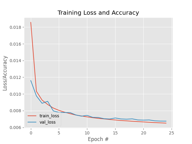
Ta thấy Train Loss và Validation Loss đều giảm dần khi số lượng epochs tăng và không xảy ra hiện tượng Overfitting.

Output code Autoencoder model, so với Input Data:

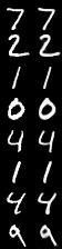
Bên trái là Input Data, còn bên phải là Output của Autoencoder model. Gần như không có sự khác biệt dữ 2 bên.

5. Kết luận

Trong bài này, chúng ta đã cùng tìm hiểu về Autoencoders, cấu tạo, cách hoạt động, ứng dụng, cũng như sự khác nhau của nó so với GAN. Chúng ta cũng đã huấn luyện một Autoencoders đơn giản trên tập MNIST.

Toàn bộ source code của bài này, các bạn có thể tham khảo tại github cá nhân của mình tại đây.

Hẹn các bạn trong các bài viết tiếp theo.

6. Tham khảo

Pyimagesearch

Autoencoder với Keras, Tensorflow và Deep Learning