SuNT's Blog | AI in Practical

Bài thứ 23 trong chuỗi các bài viết về chủ đề Data Preparation cho các mô hình ML và là bài thứ 2 về về Dimensionality Reduction. Trong bài này, chúng ta sẽ tìm hiểu về 3 thuật toán: LDA, PCA và SVD, cách sử dung chúng để thực hiện Dimensionality Reduction.

1. Linear Discriminant Analysis - LDA

LDA thực chất là một thuật toán Linear ML cho bài toán Multiclass Classification. LDA hoạt động bằng cách tìm kiếm một sự kết hợp tuyến tính giữa các features để có thể tối đa hóa khả năng phân biệt giữa các classes và tối thiểu hóa khả năng phân biệt giữa các samples trong mỗi class.

Có một thuật toán khác, cũng viết tắt là LDA. Đó là Latent Dirichlet Allocation, chuyên dùng cho Dimensionality Reduction trong bài toán Text Classification. Nhưng nó nằm ngoài phạm vi bài này, mình chỉ đưa ra đây để về sau nếu có gặp thì các bạn đỡ bối rối.

Trong scikit-learn, LDA được implemented bởi class LinearDiscriminantAnalysis(). Cách sử dụng tương tự như các kỹ thuật transforms khác. Tham số cần quan tâm là n_components chỉ ra số chiều còn lại của dữ liệu sau khi giảm. Giá trị tối đa của nó = số lượng (classes - 1).

...
# prepare dataset
data = ...
# define transform
lda = LinearDiscriminantAnalysis()
# prepare transform on dataset
lda.fit(data)
# apply transform to dataset
transformed = lda.transform(data)

Nếu sử dụng kết hợp với model trong một pipeline thì sẽ như sau:

...
# define the pipeline
steps = [('lda', LinearDiscriminantAnalysis()), ('m', GaussianNB())]
model = Pipeline(steps=steps)
...
# define the pipeline
steps = [('s', StandardScaler()), ('lda', LinearDiscriminantAnalysis()), ('m', GaussianNB())]
model = Pipeline(steps=steps)

2. Principal Component Analysis - PCA

PCA có lẽ là thuật toán Dimensionality Reduction phổ biến nhất. Khi nhắc đến Dimensionality Reduction, người ta thường nghĩ ngay đến PCA đầu tiên.

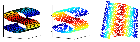
PCA hoạt động theo nguyên tắc feature projection, tức là từ m-dimension ban đầu của dữ liệu trong không gian S, thông qua một pháp ánh xạ sẽ được chuyển thành n-dimension trong không gian R mà m > n.

Trong scikit-learn, PCA được implemented bởi class PCA. Các sử dụng tương tự như các kỹ thuật transforms khác. Tham số cần chú ý của class PCA cũng là n_components như của LDA.

Cách sử dụng PCA:

...
data = ...
# define transform
pca = PCA()
# prepare transform on dataset
pca.fit(data)
# apply transform to dataset
transformed = pca.transform(data)

Nếu kết hợp với pipeline:

...
# define the pipeline
steps = [('pca', PCA()), ('m', LogisticRegression())]
model = Pipeline(steps=steps)
...
# define the pipeline
steps = [('norm', MinMaxScaler()), ('pca', PCA()), ('m', LogisticRegression())]
model = Pipeline(steps=steps)

3. Singular Value Decomposition - SVD

SVD cũng là một trong những thuật toán Dimensionality Reduction phổ biến. Cách thức hoạt động của nó tương tự như PCA, chỉ có điều nó thường được áp dụng cho các tập dữ liệu bị sparse, tức là dữ liệu mà ở đó có rất nhiều các giá trị của các features bằng 0.

Một số VD của sparse data phù hợp để áp dụng SVD là:

Recommender System
Customer-Production purchases
User-Song Listener Counts
User-Movie Ratings
Text Classification
One Hot Encoding
Bag-of-Words Counts
TF/IDF

Trong scikit-learn, SVD được implemented bởi class TruncatedSVD(). Cách sử dụng tương tự như các kỹ thuật transforms khác. Tham số cần quan tâm là n_components.

Cách sử dụng SVD:

...
data = ...
# define transform
svd = TruncatedSVD()
# prepare transform on dataset
svd.fit(data)
# apply transform to dataset
transformed = svd.transform(data)

Nếu kết hợp vào pipeline:

...
# define the pipeline
steps = [('svd', TruncatedSVD()), ('m', LogisticRegression())]
model = Pipeline(steps=steps)
...
# define the pipeline
steps = [( 'norm', MinMaxScaler()), ('svd', TruncatedSVD()), ('m', LogisticRegression())]
model = Pipeline(steps=steps)

2. Thực hành LDA, PCA và SVD

2.1 Tạo Dataset

Chúng ta sẽ tạo ra một tập gồm có 1000 mẫu dữ liệu, 10 classes, số chiều là 20, sử dụng hàm make_classification().

# test classification dataset
from sklearn.datasets import make_classification
# define dataset
X, y = make_classification(n_samples=1000, n_features=20, n_informative=15, n_redundant=5, random_state=7, n_classes=10)
# summarize the dataset
print(X.shape, y.shape)

Kết quả thực hiện:

(1000, 100) (1000,)

2.2 Thực hành LDA

a, Áp dụng LDA và Naive Bayes để mô hình hóa dữ liệu

# evaluate lda with naive bayes algorithm for classification
from numpy import mean
from numpy import std
from sklearn.datasets import make_classification
from sklearn.model_selection import cross_val_score
from sklearn.model_selection import RepeatedStratifiedKFold
from sklearn.pipeline import Pipeline
from sklearn.discriminant_analysis import LinearDiscriminantAnalysis
from sklearn.naive_bayes import GaussianNB
# define dataset
X, y = make_classification(n_samples=1000, n_features=20, n_informative=15, n_redundant=5, random_state=7, n_classes=10)
# define the pipeline
steps = [('lda', LinearDiscriminantAnalysis(n_components=5)), ('m', GaussianNB())]
model = Pipeline(steps=steps)
# evaluate model
cv = RepeatedStratifiedKFold(n_splits=10, n_repeats=3, random_state=1)
n_scores = cross_val_score(model, X, y, scoring='accuracy', cv=cv, n_jobs=-1)
# report performance
print('Accuracy: %.3f (%.3f)' % (mean(n_scores), std(n_scores)))

Kết quả thực hiện:

Accuracy: 0.366 (0.052)

b, Tune n_components của LDA

# compare lda number of components with naive bayes algorithm for classification
from numpy import mean
from numpy import std
from sklearn.datasets import make_classification
from sklearn.model_selection import cross_val_score
from sklearn.model_selection import RepeatedStratifiedKFold
from sklearn.pipeline import Pipeline
from sklearn.discriminant_analysis import LinearDiscriminantAnalysis
from sklearn.naive_bayes import GaussianNB
from matplotlib import pyplot

# get the dataset
def get_dataset():
	X, y = make_classification(n_samples=1000, n_features=20, n_informative=15, n_redundant=5, random_state=7, n_classes=10)
	return X, y

# get a list of models to evaluate
def get_models():
	models = dict()
	for i in range(1,10):
		steps = [('lda', LinearDiscriminantAnalysis(n_components=i)), ('m', GaussianNB())]
		models[str(i)] = Pipeline(steps=steps)
	return models

# evaluate a given model using cross-validation
def evaluate_model(model, X, y):
	cv = RepeatedStratifiedKFold(n_splits=10, n_repeats=3, random_state=1)
	scores = cross_val_score(model, X, y, scoring='accuracy', cv=cv, n_jobs=-1)
	return scores

# define dataset
X, y = get_dataset()
# get the models to evaluate
models = get_models()
# evaluate the models and store results
results, names = list(), list()
for name, model in models.items():
	scores = evaluate_model(model, X, y)
	results.append(scores)
	names.append(name)
	print('>%s %.3f (%.3f)' % (name, mean(scores), std(scores)))
# plot model performance for comparison
pyplot.boxplot(results, labels=names, showmeans=True)
pyplot.show()

Kết quả thực hiện:

>1 0.148 (0.030)
>2 0.209 (0.040)
>3 0.265 (0.044)
>4 0.280 (0.047)
>5 0.296 (0.051)
>6 0.324 (0.054)
>7 0.341 (0.045)
>8 0.363 (0.048)
>9 0.366 (0.052)

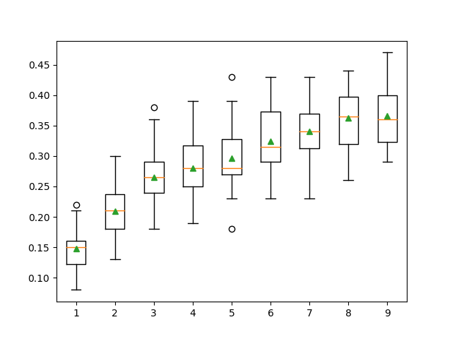
n_components=9 cho ta kết quả tốt nhất trong tất cả.

c, Dự đoán trên mẫu dữ liệu mới

# make predictions using lda with naive bayes
from sklearn.datasets import make_classification
from sklearn.pipeline import Pipeline
from sklearn.discriminant_analysis import LinearDiscriminantAnalysis
from sklearn.naive_bayes import GaussianNB
# define dataset
X, y = make_classification(n_samples=1000, n_features=20, n_informative=15, n_redundant=5, random_state=7, n_classes=10)
# define the model
steps = [('lda', LinearDiscriminantAnalysis(n_components=9)), ('m', GaussianNB())]
model = Pipeline(steps=steps)
# fit the model on the whole dataset
model.fit(X, y)
# make a single prediction
row = [[2.3548775, -1.69674567, 1.6193882, -1.19668862, -2.85422348, -2.00998376, 16.56128782, 2.57257575, 9.93779782, 0.43415008, 6.08274911, 2.12689336, 1.70100279, 3.32160983, 13.02048541, -3.05034488, 2.06346747, -3.33390362, 2.45147541, -1.23455205]]
yhat = model.predict(row)
print('Predicted Class: %d' % yhat[0])

Kết quả thực hiện:

Predicted Class: 6

2.3 Thực hành PCA

a, Áp dụng PCA và Logistic Regression để mô hình hóa dữ liệu

# evaluate pca with logistic regression algorithm for classification
from numpy import mean
from numpy import std
from sklearn.datasets import make_classification
from sklearn.model_selection import cross_val_score
from sklearn.model_selection import RepeatedStratifiedKFold
from sklearn.pipeline import Pipeline
from sklearn.decomposition import PCA
from sklearn.linear_model import LogisticRegression
# define dataset
X, y = make_classification(n_samples=1000, n_features=20, n_informative=15, n_redundant=5, random_state=7)
# define the pipeline
steps = [('pca', PCA(n_components=10)), ('m', LogisticRegression())]
model = Pipeline(steps=steps)
# evaluate model
cv = RepeatedStratifiedKFold(n_splits=10, n_repeats=3, random_state=1)
n_scores = cross_val_score(model, X, y, scoring='accuracy', cv=cv, n_jobs=-1)
# report performance
print('Accuracy: %.3f (%.3f)' % (mean(n_scores), std(n_scores)))

Kết quả thực hiện:

Accuracy: 0.816 (0.034)

b, Tune n_components của PCA

# compare pca number of components with logistic regression algorithm for classification
from numpy import mean
from numpy import std
from sklearn.datasets import make_classification
from sklearn.model_selection import cross_val_score
from sklearn.model_selection import RepeatedStratifiedKFold
from sklearn.pipeline import Pipeline
from sklearn.decomposition import PCA
from sklearn.linear_model import LogisticRegression
from matplotlib import pyplot

# get the dataset
def get_dataset():
	X, y = make_classification(n_samples=1000, n_features=20, n_informative=15, n_redundant=5, random_state=7)
	return X, y

# get a list of models to evaluate
def get_models():
	models = dict()
	for i in range(1,21):
		steps = [('pca', PCA(n_components=i)), ('m', LogisticRegression())]
		models[str(i)] = Pipeline(steps=steps)
	return models

# evaluate a given model using cross-validation
def evaluate_model(model, X, y):
	cv = RepeatedStratifiedKFold(n_splits=10, n_repeats=3, random_state=1)
	scores = cross_val_score(model, X, y, scoring='accuracy', cv=cv, n_jobs=-1)
	return scores

# define dataset
X, y = get_dataset()
# get the models to evaluate
models = get_models()
# evaluate the models and store results
results, names = list(), list()
for name, model in models.items():
	scores = evaluate_model(model, X, y)
	results.append(scores)
	names.append(name)
	print('>%s %.3f (%.3f)' % (name, mean(scores), std(scores)))
# plot model performance for comparison
pyplot.boxplot(results, labels=names, showmeans=True)
pyplot.xticks(rotation=45)
pyplot.show()

Kêt quả thực hiện:

>1 0.542 (0.048)
>2 0.713 (0.048)
>3 0.720 (0.053)
>4 0.723 (0.051)
>5 0.725 (0.052)
>6 0.730 (0.046)
>7 0.805 (0.036)
>8 0.800 (0.037)
>9 0.814 (0.036)
>10 0.816 (0.034)
>11 0.819 (0.035)
>12 0.819 (0.038)
>13 0.819 (0.035)
>14 0.853 (0.029)
>15 0.865 (0.027)
>16 0.865 (0.027)
>17 0.865 (0.027)
>18 0.865 (0.027)
>19 0.865 (0.027)
>20 0.865 (0.027)

n_components từ 15 đến 20 cho kết quả tốt nhất.

c, Tạo dự đoán trên mẫu dữ liệu mới

# make predictions using pca with logistic regression
from sklearn.datasets import make_classification
from sklearn.pipeline import Pipeline
from sklearn.decomposition import PCA
from sklearn.linear_model import LogisticRegression
# define dataset
X, y = make_classification(n_samples=1000, n_features=20, n_informative=15, n_redundant=5, random_state=7)
# define the model
steps = [('pca', PCA(n_components=15)), ('m', LogisticRegression())]
model = Pipeline(steps=steps)
# fit the model on the whole dataset
model.fit(X, y)
# make a single prediction
row = [[0.2929949, -4.21223056, -1.288332, -2.17849815, -0.64527665, 2.58097719, 0.28422388, -7.1827928, -1.91211104, 2.73729512, 0.81395695, 3.96973717, -2.66939799, 3.34692332, 4.19791821, 0.99990998, -0.30201875, -4.43170633, -2.82646737, 0.44916808]]
yhat = model.predict(row)
print('Predicted Class: %d' % yhat[0])

Kết quả thực hiện:

Predicted Class: 1

2.4 Thực hành SVD

a. Áp dụng SVD và Logistic Regression để mô hình hóa dữ liệu

# evaluate svd with logistic regression algorithm for classification
from numpy import mean
from numpy import std
from sklearn.datasets import make_classification
from sklearn.model_selection import cross_val_score
from sklearn.model_selection import RepeatedStratifiedKFold
from sklearn.pipeline import Pipeline
from sklearn.decomposition import TruncatedSVD
from sklearn.linear_model import LogisticRegression
# define dataset
X, y = make_classification(n_samples=1000, n_features=20, n_informative=15, n_redundant=5, random_state=7)
# define the pipeline
steps = [('svd', TruncatedSVD(n_components=10)), ('m', LogisticRegression())]
model = Pipeline(steps=steps)
# evaluate model
cv = RepeatedStratifiedKFold(n_splits=10, n_repeats=3, random_state=1)
n_scores = cross_val_score(model, X, y, scoring='accuracy', cv=cv, n_jobs=-1)
# report performance
print('Accuracy: %.3f (%.3f)' % (mean(n_scores), std(n_scores)))

Kết quả thực hiện:

Accuracy: 0.814 (0.034)

b, Tune n_components của SVD

# compare svd number of components with logistic regression algorithm for classification
from numpy import mean
from numpy import std
from sklearn.datasets import make_classification
from sklearn.model_selection import cross_val_score
from sklearn.model_selection import RepeatedStratifiedKFold
from sklearn.pipeline import Pipeline
from sklearn.decomposition import TruncatedSVD
from sklearn.linear_model import LogisticRegression
from matplotlib import pyplot

# get the dataset
def get_dataset():
	X, y = make_classification(n_samples=1000, n_features=20, n_informative=15, n_redundant=5, random_state=7)
	return X, y

# get a list of models to evaluate
def get_models():
	models = dict()
	for i in range(1,20):
		steps = [('svd', TruncatedSVD(n_components=i)), ('m', LogisticRegression())]
		models[str(i)] = Pipeline(steps=steps)
	return models

# evaluate a given model using cross-validation
def evaluate_model(model, X, y):
	cv = RepeatedStratifiedKFold(n_splits=10, n_repeats=3, random_state=1)
	scores = cross_val_score(model, X, y, scoring='accuracy', cv=cv, n_jobs=-1)
	return scores

# define dataset
X, y = get_dataset()
# get the models to evaluate
models = get_models()
# evaluate the models and store results
results, names = list(), list()
for name, model in models.items():
	scores = evaluate_model(model, X, y)
	results.append(scores)
	names.append(name)
	print('>%s %.3f (%.3f)' % (name, mean(scores), std(scores)))
# plot model performance for comparison
pyplot.boxplot(results, labels=names, showmeans=True)
pyplot.xticks(rotation=45)
pyplot.show()

Kết quả thực hiện:

>1 0.542 (0.046)
>2 0.626 (0.050)
>3 0.719 (0.053)
>4 0.722 (0.052)
>5 0.721 (0.054)
>6 0.729 (0.045)
>7 0.802 (0.034)
>8 0.800 (0.040)
>9 0.814 (0.037)
>10 0.814 (0.034)
>11 0.817 (0.037)
>12 0.820 (0.038)
>13 0.820 (0.036)
>14 0.825 (0.036)
>15 0.865 (0.027)
>16 0.865 (0.027)
>17 0.865 (0.027)
>18 0.865 (0.027)
>19 0.865 (0.027)

c, Tạo dự đoán trên mẫu dữ liệu mới

# make predictions using svd with logistic regression
from sklearn.datasets import make_classification
from sklearn.pipeline import Pipeline
from sklearn.decomposition import TruncatedSVD
from sklearn.linear_model import LogisticRegression
# define dataset
X, y = make_classification(n_samples=1000, n_features=20, n_informative=15, n_redundant=5, random_state=7)
# define the model
steps = [('svd', TruncatedSVD(n_components=15)), ('m', LogisticRegression())]
model = Pipeline(steps=steps)
# fit the model on the whole dataset
model.fit(X, y)
# make a single prediction
row = [[0.2929949, -4.21223056, -1.288332, -2.17849815, -0.64527665, 2.58097719, 0.28422388, -7.1827928, -1.91211104, 2.73729512, 0.81395695, 3.96973717, -2.66939799, 3.34692332, 4.19791821, 0.99990998, -0.30201875, -4.43170633, -2.82646737, 0.44916808]]
yhat = model.predict(row)
print('Predicted Class: %d' % yhat[0])

Kết quả thực hiện:

Predicted Class: 1

3. Kết luận

Bài thứ 2 về Dimensionality Reduction, chúng ta đã cùng tìm hiểu 3 thuật toán là LDA, PCA, và SVD. Chúng ta cũng đã thực hành chúng trên tập dữ liệu tự sinh. Đây cũng là bài cuối cùng trong chuỗi các bài viết về DP4ML. Hi vọng đã phần nào giúp các bạn hiểu và biết cách áp dụng các kỹ thuật đó vào quá trình chuẩn bị dữ liệu của mình để có thể tạo ra các mô hình tốt hơn.

Toàn bộ code của bài này, các bạn có thể tham khảo tại đây.

4. Tham khảo

[1] Jason Brownlee, “Data Preparation for Machine Learning”, Book: https://machinelearningmastery.com/data-preparation-for-machine-learning/.

DP4ML - Dimensionality Reduction - Phần 2 - How to Perform LDA and PCA Dimensionality Reduction

1. Linear Discriminant Analysis - LDA

2. Principal Component Analysis - PCA

3. Singular Value Decomposition - SVD

2. Thực hành LDA, PCA và SVD

2.1 Tạo Dataset

2.2 Thực hành LDA

a, Áp dụng LDA và Naive Bayes để mô hình hóa dữ liệu

b, Tune n_components của LDA

c, Dự đoán trên mẫu dữ liệu mới

2.3 Thực hành PCA

a, Áp dụng PCA và Logistic Regression để mô hình hóa dữ liệu

b, Tune n_components của PCA

c, Tạo dự đoán trên mẫu dữ liệu mới

2.4 Thực hành SVD

a. Áp dụng SVD và Logistic Regression để mô hình hóa dữ liệu

b, Tune n_components của SVD

c, Tạo dự đoán trên mẫu dữ liệu mới

3. Kết luận

4. Tham khảo